Getting Started with LSDB#
Installation#
Hint
We strongly recommend using a virtual environment. Installing packages into your system Python can create subtle problems.
Before installing the package, create and activate a fresh environment. Here are some examples with different tools:
conda create -n lsdb_env python=3.12
conda activate lsdb_env
python -m venv ./lsdb_env
source ./lsdb_env/bin/activate
With the pyenv-virtualenv plug-in:
pyenv virtualenv 3.12 lsdb_env
pyenv local lsdb_env
We recommend Python versions >=3.11, <=3.14. If you don’t have a compatible version of Python or Conda installed into your environment, and don’t have admin rights to install one, we recommend installing uv or miniforge into your user-space and creating virtual environments using these tools.
The latest release version of LSDB is available to install with pip or conda.
pip install "lsdb>=0.8.1"
conda install -c conda-forge "lsdb>=0.8.1"
LSDB can also be installed from source on GitHub. See our advanced installation instructions in the contribution guide.
Tip
There are some additional dependencies that you should install if you encounter roadblocks with the Jupyter environment or issues connecting to various remote file systems.
These can be installed with the full extra.
python -m pip install "lsdb[full]>=0.8.1"
Quickstart#
LSDB is built on top of Dask DataFrame, which allows workflows to run in parallel on distributed environments and scale to large, out-of-memory datasets. For this to work, when catalogs are opened, they are loaded lazily, meaning that only the metadata is loaded at first. This way, LSDB can plan how tasks will be executed in the future without actually doing any computation. See our tutorials for more information.
Opening a Catalog#
Let’s start by opening a HATS formatted Catalog in LSDB. Use the lsdb.open_catalog() function to
open a catalog object. We’ll pass in the URL to open the Zwicky Transient Facility Data Release 14
Catalog, and specify which columns we want to use from it.
import lsdb
ztf = lsdb.open_catalog(
    "https://data.lsdb.io/hats/ztf_dr14/ztf_object",
    columns=["ra", "dec", "ps1_objid", "nobs_r", "mean_mag_r"],
)
>> ztf
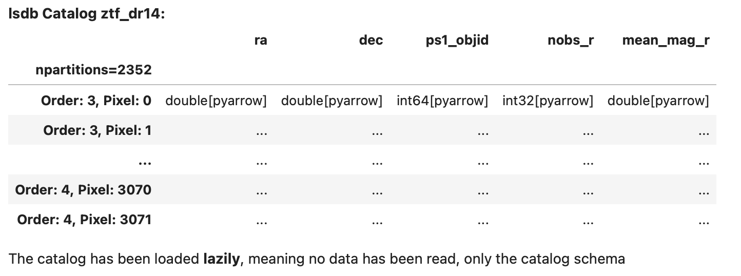
Here we can see the lazy representation of an LSDB catalog object, showing its metadata such as the column names and their types without loading any data. The rows are displayed using literal … placeholders to indicate that values are not materialized until explicitly requested.
Important
We’ve specified 5 columns to load here. It’s important for performance to select only the columns you need for your workflow. Without specifying any columns, all available columns will be loaded when the workflow is executed, making everything much slower and using much more memory.
Catalogs define a set of default columns that are loaded if you don’t specify your own list, in part
to prevent you from incurring more I/O usage than you expected. You can always see the full set
of columns available with the lsdb.catalog.Catalog.all_columns property.
Where To Get Catalogs#
LSDB can open any catalogs in the HATS format, locally or from remote sources. There are a number of catalogs available publicly to use from the cloud. You can see them with their URLs to open in LSDB at our website data.lsdb.io.
If you have your own data not in this format, you can import it by following the instructions in our importing catalogs tutorial section.
Performing Filters#
LSDB can perform spatial filters fast, taking advantage of HATS’s spatial partitioning. For the list of these
methods see the full docs for the Catalog class.
The best place to add filters is at the time of opening the catalog. This allows LSDB to avoid loading unused parts of the catalog.
lsdb.open_catalog() has keyword arguments for these filters:
search_filter=spatial filters likelsdb.ConeSearch()andlsdb.BoxSearch()
columns=column filtering (as we saw earlier)
filters=general row-based filtering expressions
The search filter narrows the catalog to include only the regions of the catalog within the spatial constraint. See the region selection tutorial for more.
ztf_cone = lsdb.open_catalog(
    catalog_path,
    search_filter=lsdb.ConeSearch(ra=40, dec=30, radius_arcsec=1000)
)
All operations on ztf_cone from here on out are constrained to the given spatial filter.
The filters= argument takes a list of lists, where each list is a condition, and all
conditions must be fulfilled for the row to make it past the filter. Below is a way
of filtering for mean_mag_r < 18 and nobs_r > 50:
ztf_rows = lsdb.open_catalog(
    catalog_path,
    filters=[["mean_mag_r", "<", 18],
             ["nobs_r", ">", 50]],

)
You can filter the catalog after it’s opened. The search filters are methods on the catalog:
ztf_cone = ztf.cone_search(ra=40, dec=30, radius_arcsec=1000)
The row-based filters on column values can be done in the same way that you would on a pandas DataFrame, using
lsdb.catalog.Catalog.query() or Pandas-like indexing expressions:
ztf_cols = ztf[["ra", "dec", "mean_mag_r", "nobs_r"]]
ztf_cone = ztf_cols.cone_search(ra=40, dec=30, radius_arcsec=1000)
ztf_filtered = ztf_cone[ztf_cone["mean_mag_r"] < 18]
ztf_filtered = ztf_filtered.query("nobs_r > 50")
Crossmatching#
Now we’ve filtered our catalog, let’s try crossmatching! We’ll need to open another catalog first.
gaia = lsdb.open_catalog(
    "https://data.lsdb.io/hats/gaia_dr3",
    columns=["ra", "dec", "phot_g_n_obs", "phot_g_mean_flux", "pm"],
)
Once we’ve got our other catalog, we can crossmatch the two together!
ztf_x_gaia = ztf_filtered.crossmatch(gaia, n_neighbors=1, radius_arcsec=3)
As with opening the catalog, this plans but does not execute the crossmatch. See the Computing section, next.
Important
Catalogs used on the right side of a crossmatch need to have a margin cache in order to get accurate
results. In the above example, Gaia DR3 is a catalog collection; opening the collection’s URL
automatically loads an appropriate margin cache. You can see what margin cache your catalog has with the
lsdb.catalog.Catalog.margin property. If it exists (is not None), you can inspect its name.
In our example, this would be gaia.margin.name.
If, when calling lsdb.catalog.Catalog.crossmatch(), you get the warning RuntimeWarning: Right
catalog does not have a margin cache. Results may be incomplete and/or inaccurate., it means that you
should provide the margin cache directly with the margin_cache= argument. You can also use this argument
to use a different margin cache than the collection’s default.
See margins tutorial section for more.
For a detailed crossmatching example, see the crossmatching tutorial.
Computing#
We’ve now planned the crossmatch lazily, but it still hasn’t been actually performed. To load the data and run
the workflow we’ll call the lsdb.catalog.Catalog.compute() method, which will perform all the tasks and
return the result as a NestedFrame with all the computed values. For more on NestedFrame (an extension
of the Pandas DataFrame) see the NestedFrame tutorial section.
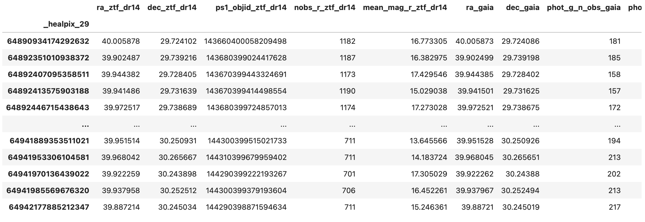
result_df = ztf_x_gaia.compute()
>> result_df
Saving the Result#
For large results, it won’t be possible to lsdb.catalog.Catalog.compute() since the full result won’t be
able to fit into memory. So instead, we can run the computation and save the results directly to disk in HATS
format.
ztf_x_gaia.write_catalog("./ztf_x_gaia")
This creates the following HATS Catalog on disk:
ztf_x_gaia/
├── dataset
│   ├── Norder=4
│   │   └── Dir=0
│   │       └── Npix=57.parquet
│   ├── _common_metadata
│   ├── _metadata
│   └── data_thumbnail.parquet
├── hats.properties
├── partition_info.csv
└── skymap.fits