RAIL photo-z estimates for Rubin Data Preview 1 (DP1)

In this tutorial, we will:

• access a photo-z catalog derived from Rubin’s Data Preview 1 using LSDB (for data rights holders)

• access the same catalog using pandas or any other Parquet reader (for all users)

• reconstruct the qp.Ensemble from the PDF nested columns

1. Loading through LSDB

In order to access the catalog through LSDB, you must be a Rubin data rights holder, because the catalog includes sky coordinates and magnitudes from the original DP1 dataset. At present, there are two ways to access this data: RSP and CANFAR, described in Accessing Rubin Data Preview 1 (DP1).

from upath import UPath
import lsdb

base_path = UPath("/rubin/lsdb_data")
dp1_pz_catalog = lsdb.open_catalog(base_path / "object_photoz")
dp1_pz_catalog

lsdb Catalog dp1_pz_wPDF:

	objectId	knn_z_median	knn_z_mean	knn_z_mode	knn_z_err95_low	knn_z_err95_high	knn_z_err68_low	knn_z_err68_high	tpz_z_median	tpz_z_mean	tpz_z_mode	tpz_z_err95_low	tpz_z_err95_high	tpz_z_err68_low	tpz_z_err68_high	cmnn_z_median	cmnn_z_mean	cmnn_z_mode	cmnn_z_err95_low	cmnn_z_err95_high	cmnn_z_err68_low	cmnn_z_err68_high	gpz_z_median	gpz_z_mean	gpz_z_mode	gpz_z_err95_low	gpz_z_err95_high	gpz_z_err68_low	gpz_z_err68_high	bpz_z_median	bpz_z_mean	bpz_z_mode	bpz_z_err95_low	bpz_z_err95_high	bpz_z_err68_low	bpz_z_err68_high	dnf_z_median	dnf_z_mean	dnf_z_mode	dnf_z_err95_low	dnf_z_err95_high	dnf_z_err68_low	dnf_z_err68_high	fzboost_z_median	fzboost_z_mean	fzboost_z_mode	fzboost_z_err95_low	fzboost_z_err95_high	fzboost_z_err68_low	fzboost_z_err68_high	lephare_z_median	lephare_z_mean	lephare_z_mode	lephare_z_err95_low	lephare_z_err95_high	lephare_z_err68_low	lephare_z_err68_high	bpz_ens_interp	cmnn_ens_norm	dnf_ens_interp	fzboost_ens_interp	knn_ens_mixmod	lephare_ens_interp	tpz_ens_interp	gpz_ens_norm	coord_ra	coord_dec
npartitions=5
Order: 3, Pixel: 2	int64[pyarrow]	double[pyarrow]	double[pyarrow]	double[pyarrow]	double[pyarrow]	double[pyarrow]	double[pyarrow]	double[pyarrow]	double[pyarrow]	double[pyarrow]	double[pyarrow]	double[pyarrow]	double[pyarrow]	double[pyarrow]	double[pyarrow]	double[pyarrow]	double[pyarrow]	double[pyarrow]	double[pyarrow]	double[pyarrow]	double[pyarrow]	double[pyarrow]	double[pyarrow]	double[pyarrow]	double[pyarrow]	double[pyarrow]	double[pyarrow]	double[pyarrow]	double[pyarrow]	double[pyarrow]	double[pyarrow]	double[pyarrow]	double[pyarrow]	double[pyarrow]	double[pyarrow]	double[pyarrow]	double[pyarrow]	double[pyarrow]	double[pyarrow]	double[pyarrow]	double[pyarrow]	double[pyarrow]	double[pyarrow]	double[pyarrow]	double[pyarrow]	double[pyarrow]	double[pyarrow]	double[pyarrow]	double[pyarrow]	double[pyarrow]	double[pyarrow]	double[pyarrow]	double[pyarrow]	double[pyarrow]	double[pyarrow]	double[pyarrow]	double[pyarrow]	nested<xvals: [double], yvals: [double]>	nested<loc: [double], scale: [double]>	nested<xvals: [double], yvals: [double]>	nested<xvals: [double], yvals: [double]>	nested<means: [double], stds: [double], weight...	nested<xvals: [double], yvals: [double]>	nested<xvals: [double], yvals: [double]>	nested<loc: [double], scale: [double]>	double[pyarrow]	double[pyarrow]
Order: 5, Pixel: 4471	...	...	...	...	...	...	...	...	...	...	...	...	...	...	...	...	...	...	...	...	...	...	...	...	...	...	...	...	...	...	...	...	...	...	...	...	...	...	...	...	...	...	...	...	...	...	...	...	...	...	...	...	...	...	...	...	...	...	...	...	...	...	...	...	...	...	...
Order: 2, Pixel: 80	...	...	...	...	...	...	...	...	...	...	...	...	...	...	...	...	...	...	...	...	...	...	...	...	...	...	...	...	...	...	...	...	...	...	...	...	...	...	...	...	...	...	...	...	...	...	...	...	...	...	...	...	...	...	...	...	...	...	...	...	...	...	...	...	...	...	...
Order: 3, Pixel: 536	...	...	...	...	...	...	...	...	...	...	...	...	...	...	...	...	...	...	...	...	...	...	...	...	...	...	...	...	...	...	...	...	...	...	...	...	...	...	...	...	...	...	...	...	...	...	...	...	...	...	...	...	...	...	...	...	...	...	...	...	...	...	...	...	...	...	...
Order: 3, Pixel: 561	...	...	...	...	...	...	...	...	...	...	...	...	...	...	...	...	...	...	...	...	...	...	...	...	...	...	...	...	...	...	...	...	...	...	...	...	...	...	...	...	...	...	...	...	...	...	...	...	...	...	...	...	...	...	...	...	...	...	...	...	...	...	...	...	...	...	...

67 out of 67 available columns in the catalog have been loaded lazily, meaning no data has been read, only the catalog schema

2. Loading through single parquet

The photo-z parquet is available to everyone.

import pandas as pd

dp1_pz_df = pd.read_parquet("https://data.lsdb.io/hats/dp1/object_photoz.parquet")
dp1_pz_df

	objectId	lephare_z_median	lephare_z_mean	lephare_z_mode	lephare_z_err95_low	lephare_z_err95_high	lephare_z_err68_low	lephare_z_err68_high	knn_z_median	knn_z_mode	...	dnf_z_err95_high	dnf_z_err68_low	dnf_z_err68_high	fzboost_z_median	fzboost_z_mean	fzboost_z_mode	fzboost_z_err95_low	fzboost_z_err95_high	fzboost_z_err68_low	fzboost_z_err68_high
0	648368263004160627	0.472849	1.006352	0.26	0.025956	2.928256	0.189219	2.262542	0.354946	0.35	...	1.930399	0.307735	1.813800	1.470184	1.688171	1.45	0.190596	2.899186	1.213509	2.837311
1	648368263004160629	0.797163	0.798260	0.79	0.608637	0.971621	0.706346	0.888711	0.870491	0.83	...	2.416718	0.805785	2.290113	0.909653	0.932351	0.89	0.776280	1.305105	0.846703	1.019736
...	...	...	...	...	...	...	...	...	...	...	...	...	...	...	...	...	...	...	...	...	...
544642	614438364963147249	0.589314	0.594391	0.60	0.418283	0.749071	0.506786	0.664330	0.675214	0.68	...	0.841858	0.422715	0.742535	0.676110	0.675869	0.69	0.576561	0.763610	0.621661	0.723309
544643	614438364963147782	1.622839	1.480223	0.37	0.029293	2.956957	0.255455	2.733078	0.673305	0.75	...	1.608661	1.126678	1.506282	2.403406	1.966630	2.88	0.229808	2.916787	0.290888	2.883602

544644 rows × 56 columns

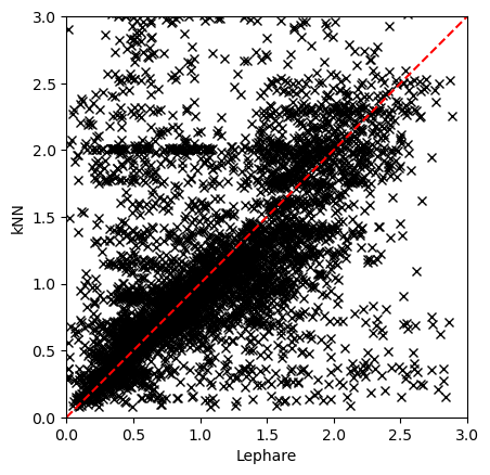
Plotting two estimators

Plotting, as an example, the results from Lephare and kNN.

import matplotlib.pyplot as plt

plt.plot(dp1_pz_df["lephare_z_median"].iloc[::100], dp1_pz_df["knn_z_median"].iloc[::100], "x", color="black")
plt.gca().set_aspect("equal", adjustable="box")
plt.plot([0, 3], [0, 3], color="red", ls="--")
plt.xlim([0, 3])
plt.ylim([0, 3])
plt.xlabel("Lephare")
plt.ylabel("kNN")

Text(0, 0.5, 'kNN')

3. Reconstructing a QP Ensemble

Here we demonstrate how to reconstruct a dictionary of qp.Ensemble objects from the HATS catalog.

Based on the column suffix (e.g., interp, mixmod, norm, hist, or quantile lengths like 99, 20, 5), we parse the nested data fields and rebuild each ensemble using the appropriate qp generator.

import qp
import numpy as np


def hats_to_qp(df):
    """Reconstruct `qp.Ensemble` objects from a partition."""
    ensembles = {}

    def extract(nf, subcol):
        return np.asarray([i[subcol] for i in nf])

    for col in df.nested_columns:
        nf = df[col]
        data_dict = {}
        ens_type = col.split("_")[-1]

        match ens_type:
            case "interp":
                data_dict["yvals"] = extract(nf, "yvals")
                data_dict["xvals"] = np.asarray(nf.iloc[-1]["xvals"])
                gen_class = qp.interp_gen
            case "mixmod":
                data_dict["means"] = extract(nf, "means")
                data_dict["stds"] = extract(nf, "stds")
                data_dict["weights"] = extract(nf, "weights")
                gen_class = qp.mixmod_gen
            case "norm":
                data_dict["loc"] = extract(nf, "loc")
                data_dict["scale"] = extract(nf, "scale")
                ensembles[col] = qp.Ensemble(qp.stats.norm, data=data_dict)
                gen_class = qp.stats.norm
            case "hist":
                data_dict["pdfs"] = extract(nf, "pdfs")
                data_dict["bins"] = np.linspace(0, 3, 301)
                gen_class = qp.hist_gen
            case "99" | "20" | "5":
                data_dict["locs"] = extract(nf, "locs")
                data_dict["quants"] = np.asarray(nf.iloc[-1]["quants"])
                gen_class = qp.quant_gen
            case _:
                continue

        ensembles[col] = qp.Ensemble(gen_class, data=data_dict)

    return ensembles

Notice that computing the qp.Ensemble is very computationally expensive. For demonstration purposes we only used a handful of objects.

hats_to_qp(dp1_pz_catalog.head())

{'bpz_ens_interp': Ensemble(the_class=interp,shape=(5, 301)),
 'cmnn_ens_norm': Ensemble(the_class=norm,shape=(5, 1)),
 'dnf_ens_interp': Ensemble(the_class=interp,shape=(5, 301)),
 'fzboost_ens_interp': Ensemble(the_class=interp,shape=(5, 301)),
 'knn_ens_mixmod': Ensemble(the_class=mixmod,shape=(5, 10)),
 'lephare_ens_interp': Ensemble(the_class=interp,shape=(5, 301)),
 'tpz_ens_interp': Ensemble(the_class=interp,shape=(5, 301)),
 'gpz_ens_norm': Ensemble(the_class=norm,shape=(5, 1))}

About

Authors: Sandro Campos, Sarah Pelesky, Tianqing Zhang

Last run: Jan 29, 2026

If you use lsdb for published research, please cite following instructions.