Region Selection#
In this tutorial, we will:
set up a Dask client and load an object catalog
select data from regions in the sky using
cone
RA/Dec box
polygon
constructed MOC (multi-order coverage map)
Introduction#
Large astronomical surveys contain a massive volume of data. Billion-object, multi-terabyte-sized catalogs are challenging to store and manipulate because they demand state-of-the-art hardware. Processing them is expensive, both in terms of runtime and memory consumption, and doing so on a single machine has become impractical. LSDB is a solution that enables scalable algorithm execution. It handles loading, querying, filtering, and crossmatching astronomical data (of HATS format) in a distributed environment.
[1]:
import lsdb
1. Load a catalog#
We create a basic dask client, and load an existing HATS catalog - the ZTF DR22 catalog.
Additional Help
For additional information on dask client creation, please refer to the official Dask documentation and our Dask cluster configuration page for LSDB-specific tips. Note that dask also provides its own best practices, which may also be useful to consult.
For tips on accessing remote data, see our Accessing remote data guide
[2]:
from dask.distributed import Client

client = Client(n_workers=4, memory_limit="auto")
client
[2]:
Client
Client-48c1246b-232f-11f1-95c2-8e6cf3dc31f8
| Connection method: Cluster object | Cluster type: distributed.LocalCluster |
| Dashboard: http://127.0.0.1:8787/status |
Cluster Info
LocalCluster
a6e43b20
| Dashboard: http://127.0.0.1:8787/status | Workers: 4 |
| Total threads: 4 | Total memory: 13.09 GiB |
| Status: running | Using processes: True |
Scheduler Info
Scheduler
Scheduler-889583d1-0581-4edf-be22-11cd751d5e24
| Comm: tcp://127.0.0.1:45775 | Workers: 0 |
| Dashboard: http://127.0.0.1:8787/status | Total threads: 0 |
| Started: Just now | Total memory: 0 B |
Workers
Worker: 0
| Comm: tcp://127.0.0.1:44499 | Total threads: 1 |
| Dashboard: http://127.0.0.1:37837/status | Memory: 3.27 GiB |
| Nanny: tcp://127.0.0.1:42921 | |
| Local directory: /tmp/dask-scratch-space/worker-4v9jm0o5 | |
Worker: 1
| Comm: tcp://127.0.0.1:45045 | Total threads: 1 |
| Dashboard: http://127.0.0.1:38725/status | Memory: 3.27 GiB |
| Nanny: tcp://127.0.0.1:37675 | |
| Local directory: /tmp/dask-scratch-space/worker-wan37kxq | |
Worker: 2
| Comm: tcp://127.0.0.1:41405 | Total threads: 1 |
| Dashboard: http://127.0.0.1:44879/status | Memory: 3.27 GiB |
| Nanny: tcp://127.0.0.1:40667 | |
| Local directory: /tmp/dask-scratch-space/worker-ypqoqmqa | |
Worker: 3
| Comm: tcp://127.0.0.1:35105 | Total threads: 1 |
| Dashboard: http://127.0.0.1:34227/status | Memory: 3.27 GiB |
| Nanny: tcp://127.0.0.1:42561 | |
| Local directory: /tmp/dask-scratch-space/worker-fuinizcq | |
[3]:
ztf_object_path = "https://data.lsdb.io/hats/ztf_dr22/ztf_lc"
ztf_object = lsdb.open_catalog(ztf_object_path)
ztf_object
[3]:
| objectid | filterid | objra | objdec | nepochs | hmjd | mag | magerr | clrcoeff | catflags | |
|---|---|---|---|---|---|---|---|---|---|---|
| npartitions=10839 | ||||||||||
| Order: 4, Pixel: 0 | int64[pyarrow] | int8[pyarrow] | float[pyarrow] | float[pyarrow] | int64[pyarrow] | list<element: double>[pyarrow] | list<element: float>[pyarrow] | list<element: float>[pyarrow] | list<element: float>[pyarrow] | list<element: int32>[pyarrow] |
| Order: 4, Pixel: 1 | ... | ... | ... | ... | ... | ... | ... | ... | ... | ... |
| ... | ... | ... | ... | ... | ... | ... | ... | ... | ... | ... |
| Order: 5, Pixel: 12286 | ... | ... | ... | ... | ... | ... | ... | ... | ... | ... |
| Order: 5, Pixel: 12287 | ... | ... | ... | ... | ... | ... | ... | ... | ... | ... |
2. Selecting a region of the sky#
There are 3 common types of spatial filters to select a portion of the sky: cone, polygon and box.
Filtering consists of two main steps:
A coarse stage, in which we find what pixels cover our desired region in the sky. These may overlap with the region and only be partially contained within the region boundaries. This means that some data points inside that pixel may fall outside of the region.
A fine stage, where we filter the data points from each pixel to make sure they fall within the specified region.
The fine parameter allows us to specify whether or not we desire to run the fine stage, for each search. It brings some overhead, so if your intention is to get a rough estimate of the data points for a region, you may disable it. It is always executed by default.
catalog.box_search(..., fine=False)
catalog.cone_search(..., fine=False)
catalog.polygon_search(..., fine=False)
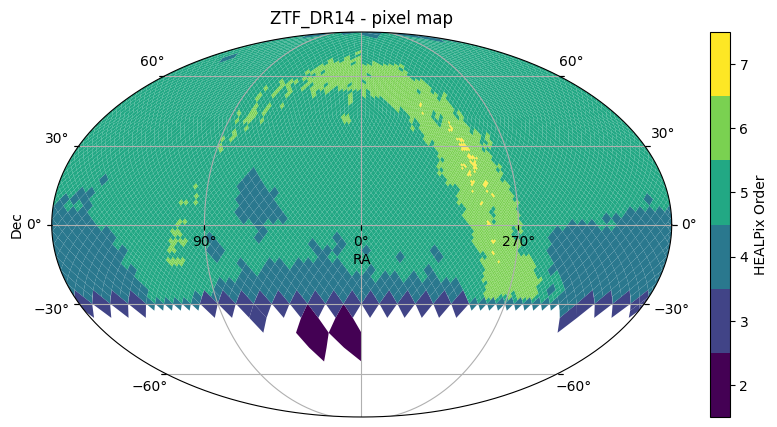
Throughout this notebook, we will use the Catalog’s plot_pixels method to display the HEALPix of each resulting catalog as filters are applied.
[4]:
ztf_object.plot_pixels(plot_title="ZTF_DR14 - pixel map")
[4]:
(<Figure size 1000x500 with 2 Axes>,
 <WCSAxes: title={'center': 'ZTF_DR14 - pixel map'}>)
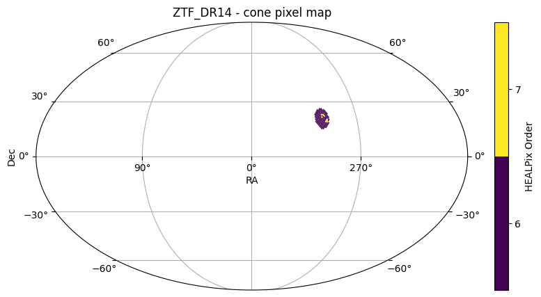
3. Cone search#
A cone search is defined by center (ra, dec), in degrees, and radius r, in arcseconds.
[5]:
ztf_object_cone = ztf_object.cone_search(ra=-60.3, dec=20.5, radius_arcsec=5 * 3600)
ztf_object_cone
[5]:
| objectid | filterid | objra | objdec | nepochs | hmjd | mag | magerr | clrcoeff | catflags | |
|---|---|---|---|---|---|---|---|---|---|---|
| npartitions=142 | ||||||||||
| Order: 6, Pixel: 12843 | int64[pyarrow] | int8[pyarrow] | float[pyarrow] | float[pyarrow] | int64[pyarrow] | list<element: double>[pyarrow] | list<element: float>[pyarrow] | list<element: float>[pyarrow] | list<element: float>[pyarrow] | list<element: int32>[pyarrow] |
| Order: 6, Pixel: 12844 | ... | ... | ... | ... | ... | ... | ... | ... | ... | ... |
| ... | ... | ... | ... | ... | ... | ... | ... | ... | ... | ... |
| Order: 6, Pixel: 14400 | ... | ... | ... | ... | ... | ... | ... | ... | ... | ... |
| Order: 6, Pixel: 14401 | ... | ... | ... | ... | ... | ... | ... | ... | ... | ... |
[6]:
ztf_object_cone.plot_pixels(plot_title="ZTF_DR14 - cone pixel map")
[6]:
(<Figure size 1000x500 with 2 Axes>,
 <WCSAxes: title={'center': 'ZTF_DR14 - cone pixel map'}>)
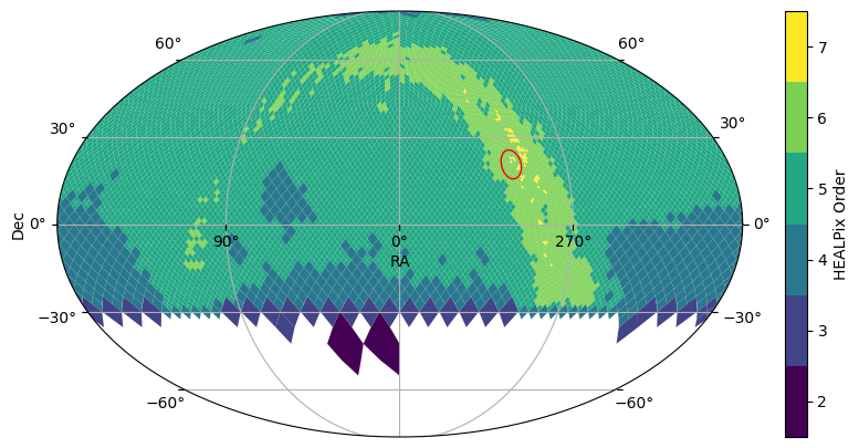
4. The Search object#
To perform a search on a catalog, there are two modes: a shape-specific call, or passing a search object to the search() method. The above case uses the cone shape call.
Using a search object can be useful if you intend to re-use the shape for filtering multiple catalogs. We also provide some basic plotting for cone and box searches. The 5 degree cone search is outlined in red in the below plot.
[7]:
from lsdb import ConeSearch

cone_search = ConeSearch(ra=-60.3, dec=20.5, radius_arcsec=5 * 3600)
[8]:
ztf_object.plot_pixels(plot_title="ZTF_DR14 - pixel map")
cone_search.plot(fc="#00000000", ec="red")
[8]:
(<Figure size 1000x500 with 2 Axes>, <WCSAxes: >)
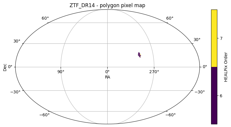
5. Polygon search#
A polygon search is defined by convex polygon with vertices [(ra1, dec1), (ra2, dec2)...], in degrees.
[9]:
vertices = [(-60.5, 15.1), (-62.5, 18.5), (-65.2, 15.3), (-64.2, 12.1)]
ztf_object_polygon = ztf_object.polygon_search(vertices)
ztf_object_polygon
[9]:
| objectid | filterid | objra | objdec | nepochs | hmjd | mag | magerr | clrcoeff | catflags | |
|---|---|---|---|---|---|---|---|---|---|---|
| npartitions=35 | ||||||||||
| Order: 6, Pixel: 12842 | int64[pyarrow] | int8[pyarrow] | float[pyarrow] | float[pyarrow] | int64[pyarrow] | list<element: double>[pyarrow] | list<element: float>[pyarrow] | list<element: float>[pyarrow] | list<element: float>[pyarrow] | list<element: int32>[pyarrow] |
| Order: 6, Pixel: 12843 | ... | ... | ... | ... | ... | ... | ... | ... | ... | ... |
| ... | ... | ... | ... | ... | ... | ... | ... | ... | ... | ... |
| Order: 7, Pixel: 122748 | ... | ... | ... | ... | ... | ... | ... | ... | ... | ... |
| Order: 7, Pixel: 122749 | ... | ... | ... | ... | ... | ... | ... | ... | ... | ... |
[10]:
ztf_object_polygon.plot_pixels(plot_title="ZTF_DR14 - polygon pixel map")
[10]:
(<Figure size 1000x500 with 2 Axes>,
 <WCSAxes: title={'center': 'ZTF_DR14 - polygon pixel map'}>)
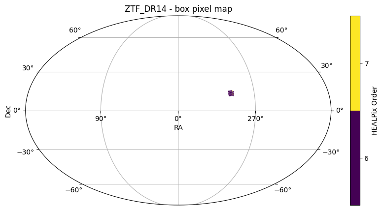
6. Box search#
A box search can be defined by right ascension and declination bands [(ra1, ra2), (dec1, dec2)].
[11]:
ztf_object_box = ztf_object.box_search(ra=[-65, -60], dec=[12, 15])
ztf_object_box
[11]:
| objectid | filterid | objra | objdec | nepochs | hmjd | mag | magerr | clrcoeff | catflags | |
|---|---|---|---|---|---|---|---|---|---|---|
| npartitions=36 | ||||||||||
| Order: 6, Pixel: 12834 | int64[pyarrow] | int8[pyarrow] | float[pyarrow] | float[pyarrow] | int64[pyarrow] | list<element: double>[pyarrow] | list<element: float>[pyarrow] | list<element: float>[pyarrow] | list<element: float>[pyarrow] | list<element: int32>[pyarrow] |
| Order: 6, Pixel: 12840 | ... | ... | ... | ... | ... | ... | ... | ... | ... | ... |
| ... | ... | ... | ... | ... | ... | ... | ... | ... | ... | ... |
| Order: 7, Pixel: 122737 | ... | ... | ... | ... | ... | ... | ... | ... | ... | ... |
| Order: 7, Pixel: 122738 | ... | ... | ... | ... | ... | ... | ... | ... | ... | ... |
[12]:
ztf_object_box.plot_pixels(plot_title="ZTF_DR14 - box pixel map")
[12]:
(<Figure size 1000x500 with 2 Axes>,
 <WCSAxes: title={'center': 'ZTF_DR14 - box pixel map'}>)
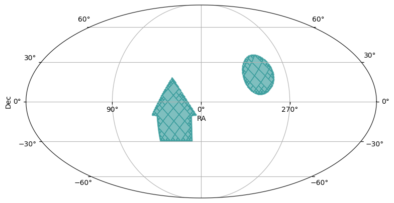
7. Complex and MOC filters#
We can stack a several number of filters, which are applied in sequence. For example, catalog.box_search().polygon_search() should result in a perfectly valid HATS catalog containing the objects that match both filters.
However, we can also get the MOC (or Multi-Order coverage map) of the regions, and perform a filter based on that region. Check out our notebook on constructing complex regions in a MOC in the HATS documentation. Here, we will use similar regions as that notebook.
However, we set the max_depth to the same granularity as the highest HEALPix order in our catalog. This ensures that we’re not getting data partitions that are completely outside of the regions, just due to low resolution MOCs.
[13]:
from hats.pixel_math import region_to_moc
from hats.inspection.visualize_catalog import plot_moc

max_depth = ztf_object.hc_structure.get_max_coverage_order()

box_moc = region_to_moc.box_to_moc(ra=[10, 45], dec=[-30, -5], max_depth=max_depth)
cone_moc = region_to_moc.cone_to_moc(ra=-60.3, dec=20.5, radius_arcsec=15 * 3600, max_depth=max_depth)
polygon_moc = region_to_moc.polygon_to_moc([(5, -10), (50, -10), (30, 18)], max_depth=max_depth)
union_moc = polygon_moc.union(cone_moc, box_moc)
plot_moc(union_moc)
[13]:
(<Figure size 900x500 with 1 Axes>, <WCSAxes: >)
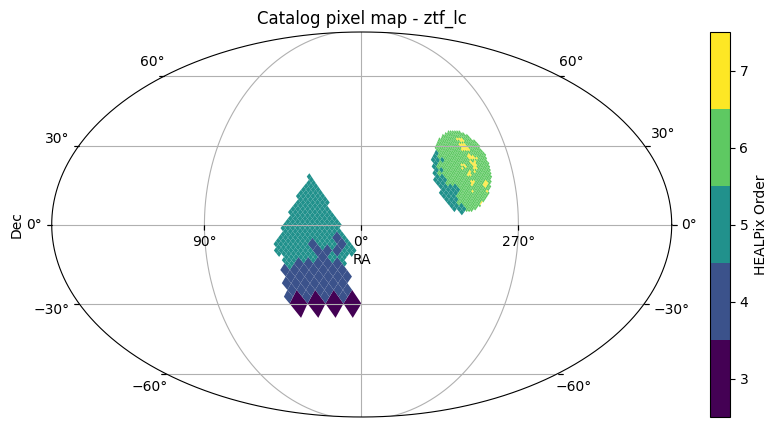
[14]:
ztf_object_moc = ztf_object.moc_search(union_moc)
ztf_object_moc
[14]:
| objectid | filterid | objra | objdec | nepochs | hmjd | mag | magerr | clrcoeff | catflags | |
|---|---|---|---|---|---|---|---|---|---|---|
| npartitions=1247 | ||||||||||
| Order: 5, Pixel: 10 | int64[pyarrow] | int8[pyarrow] | float[pyarrow] | float[pyarrow] | int64[pyarrow] | list<element: double>[pyarrow] | list<element: float>[pyarrow] | list<element: float>[pyarrow] | list<element: float>[pyarrow] | list<element: int32>[pyarrow] |
| Order: 5, Pixel: 32 | ... | ... | ... | ... | ... | ... | ... | ... | ... | ... |
| ... | ... | ... | ... | ... | ... | ... | ... | ... | ... | ... |
| Order: 5, Pixel: 9214 | ... | ... | ... | ... | ... | ... | ... | ... | ... | ... |
| Order: 5, Pixel: 9215 | ... | ... | ... | ... | ... | ... | ... | ... | ... | ... |
[15]:
ztf_object_moc.plot_pixels()
[15]:
(<Figure size 1000x500 with 2 Axes>,
 <WCSAxes: title={'center': 'Catalog pixel map - ztf_lc'}>)
Closing the Dask client#
[16]:
client.close()
About#
Authors: Sandro Campos and Melissa DeLucchi
Last updated on: August 29, 2025
If you use lsdb for published research, please cite following instructions.