Crossmatching Catalogs

In this tutorial, we will:

• test a crossmatch by limiting inputs using cone searches and column selection

• crossmatch objects between two catalogs using ra and dec

• apply margin caches during crossmatching and evaluate the default margin cache configuration

Introduction

To crossmatch two catalogs is to create a new catalog that contains columns from both inputs, with the rows aligned based on the geometric match of their ra and dec columns.

import lsdb
from dask.distributed import Client

1. Open a catalog

We create a basic dask client, and open an existing HATS catalog—the ZTF DR22 catalog.

Additional Help

For additional information on dask client creation, please refer to the official Dask documentation and our Dask cluster configuration page for LSDB-specific tips. Note that dask also provides its own best practices, which may also be useful to consult.

For tips on accessing remote data, see our Accessing remote data guide.

Create a basic Dask client, limiting the number of workers. This keeps subsequent operations from using more of our compute resources than we might intend, which is helpful in any case but especially when working on a shared resource.

client = Client(n_workers=4, memory_limit="auto")

We open two catalogs, ZTF DR22 and Gaia DR3. Both of these are catalog collections on http://data.lsdb.io, and each of them has a default margin cache catalog that is implicitly loaded. The margin cache is important for crossmatching, as it will help with cases when objects of interest are right at the edge of the catalog pixels.

See the margins tutorial for more on the importance of the margin cache.

ztf22 = lsdb.open_catalog(
    "https://data.lsdb.io/hats/ztf_dr22",
)

gaia3 = lsdb.open_catalog(
    "https://data.lsdb.io/hats/gaia_dr3",
)

display(ztf22.columns)
display(gaia3.columns)

Index(['objectid', 'filterid', 'fieldid', 'rcid', 'objra', 'objdec', 'nepochs',
       'hmjd', 'mag', 'magerr', 'clrcoeff', 'catflags', 'Norder', 'Dir',
       'Npix'],
      dtype='object')

Index(['solution_id', 'designation', 'source_id', 'random_index', 'ref_epoch',
       'ra', 'ra_error', 'dec', 'dec_error', 'parallax',
       ...
       'azero_gspphot', 'azero_gspphot_lower', 'azero_gspphot_upper',
       'ag_gspphot', 'ag_gspphot_lower', 'ag_gspphot_upper',
       'ebpminrp_gspphot', 'ebpminrp_gspphot_lower', 'ebpminrp_gspphot_upper',
       'libname_gspphot'],
      dtype='object', length=152)

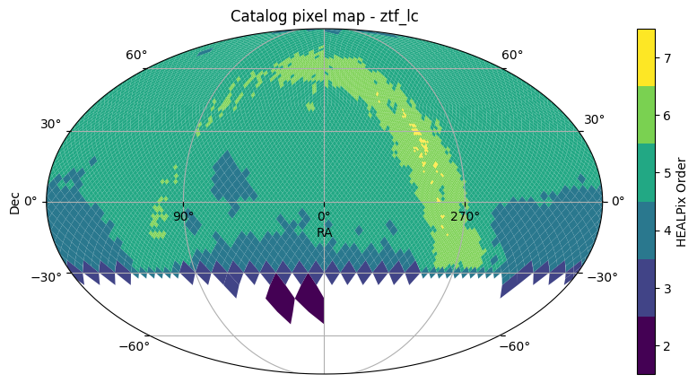
1.1 Will these catalogs have any overlap at all?

To find an area of the sky where we know that crossmatching will succeed, we can use .plot_pixels() to get a quick view of the sky coverage for each catalog.

ztf22.plot_pixels()

(<Figure size 1000x500 with 2 Axes>,
 <WCSAxes: title={'center': 'Catalog pixel map - ztf_lc'}>)

gaia3.plot_pixels()

(<Figure size 1000x500 with 2 Axes>,
 <WCSAxes: title={'center': 'Catalog pixel map - gaia'}>)

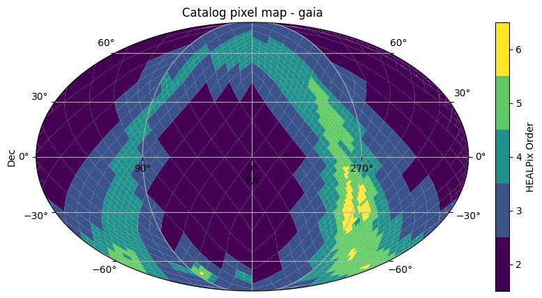
Yes, looks like they will, above dec=-30.

1.2 Work with small sections of the catalogs first

Before firing up the whole compute cluster to match both catalogs, it’s good practice to choose a small section of each catalog first, greatly limiting both I/O and compute. We can limit spatially by using a search filter such as a cone search or box search, and can limit structurally by only loading columns of interest.

Let’s use a cone search to isolate a tiny part of both catalogs in the same area, so that we can test our crossmatch. We’ll set the search filters of both catalogs to lsdb.ConeSearch(280, 0, radius_arcsec=36).

We’ll use the suffix _sm (small) to distinguish these from the full catalog.

ztf22_sm = lsdb.open_catalog(
    "https://data.lsdb.io/hats/ztf_dr22",
    columns=["objectid", "objra", "objdec", "nepochs", "hmjd", "mag", "magerr"],
    search_filter=lsdb.ConeSearch(280, 0, radius_arcsec=36),
)
ztf22_sm

lsdb Catalog ztf_lc:

	objectid	objra	objdec	nepochs	hmjd	mag	magerr
npartitions=1
Order: 6, Pixel: 30357	int64[pyarrow]	float[pyarrow]	float[pyarrow]	int64[pyarrow]	list<element: double>[pyarrow]	list<element: float>[pyarrow]	list<element: float>[pyarrow]

7 out of 15 columns in the catalog have been loaded lazily, meaning no data has been read, only the catalog schema

1.3 Nesting columns with list data

Note that ZTF DR22 has lightcurve data stored as lists under each column. To access and crossmatch these efficiently, we will use .nest_lists to arrange these lists into a single “nest” in the catalog.

For more information on nested data, see the NestedFrame tutorial.

Three of the loaded columns in ztf_lc are of type list, so let’s put those lists into a nest named lc, to make them more tractable.

ztf22_sm = ztf22_sm.nest_lists(
    list_columns=["hmjd", "mag", "magerr"],
    name="lc",
)
ztf22_sm

lsdb Catalog ztf_lc:

	objectid	objra	objdec	nepochs	lc
npartitions=1
Order: 6, Pixel: 30357	int64[pyarrow]	float[pyarrow]	float[pyarrow]	int64[pyarrow]	nested<hmjd: [double], mag: [float], magerr: [...

5 out of 15 columns in the catalog have been loaded lazily, meaning no data has been read, only the catalog schema

This small version, which we call ztf22_sm, occupies only one partition. Pulling this into memory with .compute() won’t take too long.

We’re interested in seeing how many objects are in our chosen cone search. The catalog identifiers for ZTF (objectid) and Gaia (source_id) are unique, one row for each, so the count of rows tells us the number of objects.

%%time
ztf_cone_objs = ztf22_sm["objectid"].compute()
print("Unique ZTF objects in the cone:", len(ztf_cone_objs))

Unique ZTF objects in the cone: 129
CPU times: user 2.09 s, sys: 1.09 s, total: 3.19 s
Wall time: 47.5 s

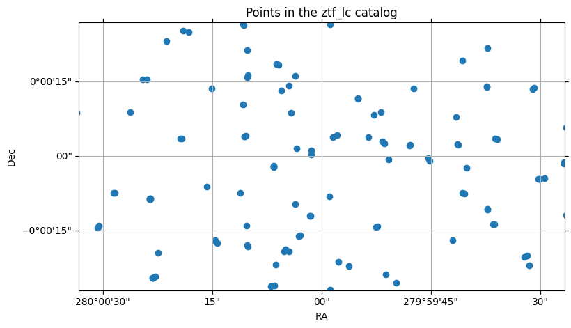
1.4 Viewing the objects within the cone searches

We can plot these points graphically:

%%time
from astropy.coordinates import SkyCoord
import astropy.units as u

# Center our view on the cone.
center = SkyCoord(280 * u.deg, 0 * u.deg)
fov = (1 * u.arcmin, 1 * u.arcmin)

ztf22_sm.plot_points(center=center, fov=fov)

CPU times: user 1.72 s, sys: 853 ms, total: 2.57 s
Wall time: 38.1 s

(<Figure size 900x500 with 1 Axes>,
 <WCSAxes: title={'center': 'Points in the ztf_lc catalog'}>)

Now let’s treat the Gaia catalog the same way, using the same small cone search, and selecting only a few columns of interest. Again, we’ll use the suffix _sm for “small”:

gaia3_sm = lsdb.open_catalog(
    "https://data.lsdb.io/hats/gaia_dr3",
    columns=["source_id", "ra", "dec", "parallax", "phot_g_n_obs", "phot_g_mean_mag"],
    search_filter=lsdb.ConeSearch(280, 0, radius_arcsec=36),
)
gaia3_sm

lsdb Catalog gaia:

	source_id	ra	dec	parallax	phot_g_n_obs	phot_g_mean_mag
npartitions=1
Order: 4, Pixel: 1897	int64[pyarrow]	double[pyarrow]	double[pyarrow]	double[pyarrow]	int16[pyarrow]	float[pyarrow]

6 out of 152 columns in the catalog have been loaded lazily, meaning no data has been read, only the catalog schema

%%time
gaia_cone_objs = gaia3_sm["source_id"].compute()
print("Unique Gaia sources in the cone:", len(gaia_cone_objs))

Unique Gaia sources in the cone: 17
CPU times: user 472 ms, sys: 237 ms, total: 709 ms
Wall time: 9.97 s

%%time
gaia3_sm.plot_points(center=center, fov=fov)

CPU times: user 552 ms, sys: 230 ms, total: 783 ms
Wall time: 10.7 s

(<Figure size 900x500 with 1 Axes>,
 <WCSAxes: title={'center': 'Points in the gaia catalog'}>)

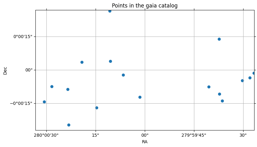
We can see that the Gaia catalog is much more sparse than the ZTF catalog, having almost a tenth of the objects for the same area of the sky.

2. Perform the crossmatch on the small catalogs

The default crossmatch algorithm is the KdTreeCrossmatch, and it is performed in a manner similar to an inner join, in that the resulting catalog will only have rows containing objects that exist in both catalogs. This also means that only pixels common to both catalogs are used in the crossmatch; you don’t need to arrange this yourself.

2.1 Effect of ordering on crossmatching

However, this doesn’t mean that the order of the catalogs doesn’t matter. As we’ll see, gaia X ztf gives us different results than ztf X gaia, even though the unique objects from the two catalogs participating in the crossmatch remain the same.

The algorithm takes each object in the left catalog and finds the closest spatial match from the right catalog.

If the left catalog is denser, this means that we are more likely to have objects from the left matching the same object on the right, giving us more rows. If the left catalog is sparser, we are more likely to have objects in the left with no matches on the right, and therefore the result may have fewer rows, as in the next example.

2.1.1 gaia X ztf (sparser on the left)

We’ll start by matching Gaia against ZTF, or gaia X ztf. Note that gaia_x_ztf will be the uncomputed catalog, and we’ll use the prefix c_, or c_gaia_x_ztf to indicate the computed result. The computed result from this small crossmatch will fit easily in memory, and it will be a NestedFrame.

%%time
gaia_x_ztf = gaia3_sm.crossmatch(ztf22_sm)
c_gaia_x_ztf = gaia_x_ztf.compute()
c_gaia_x_ztf

CPU times: user 3.4 s, sys: 1.12 s, total: 4.53 s
Wall time: 49.7 s

	source_id_gaia	ra_gaia	dec_gaia	parallax_gaia	phot_g_n_obs_gaia	phot_g_mean_mag_gaia	objectid_ztf_lc	objra_ztf_lc	objdec_ztf_lc	nepochs_ztf_lc	lc_ztf_lc	_dist_arcsec
2136230505053742297	4272460980177200768	280.000432	-0.003361	0.306259	102	20.670609	435213300004409	280.000427	-0.003351	100	hmjd mag magerr 58280.34025 21.346365 0.202767 +99 rows ... ...	0.038935
2136230505911963019	4272460980182044416	279.993450	-0.003846		61	20.738001	435313300048086	279.993469	-0.003805	144	hmjd mag magerr 58956.44194 19.609255 0.094674 +143 rows ... ...	0.162300
2136230507990852146	4272461018841217920	280.006446	-0.006851	-0.070988	164	20.329275	1481208400000483	280.006409	-0.006818	18	hmjd mag magerr 59424.35363 20.744385 0.156009 +17 rows ... ...	0.155598
2136230510106305823	4272461018829177728	280.004081	-0.004709	-0.233567	147	20.310305	435213300027218	280.004059	-0.004711	475	hmjd mag magerr 58217.48498 20.739437 0.160214 +474 rows ... ...	0.040958
2136230510539474332	4272461018841218432	280.008516	-0.003975	-0.642788	126	20.438658	435213300004426	280.008514	-0.003947	271	hmjd mag magerr 58256.46163 21.080118 0.1841 +270 rows ... ...	0.105025
2136230511149475917	4272461014544179712	280.007883	-0.002041	0.824229	93	20.665417	435313300153496	280.007874	-0.002036	131	hmjd mag magerr 58955.48525 19.965302 0.120152 +130 rows ... ...	0.061448
2136230511175473210	4272461018841219072	280.006530	-0.002397	0.474788	179	15.848508	435313300083253	280.006531	-0.002385	174	hmjd mag magerr 58955.48525 14.938301 0.017674 +173 rows ... ...	0.043069
2136230517889181962	4272461014537456000	280.005341	0.000974	0.752347	173	19.777922	435213300004315	280.005341	0.000983	498	hmjd mag magerr 58218.50632 20.483944 0.141925 +497 rows ... ...	0.059946
2136230518300361978	4272461014536964480	280.001820	-0.000606	0.135197	175	18.720890	435313300008254	280.001831	-0.000595	174	hmjd mag magerr 58955.48525 17.876301 0.031538 +173 rows ... ...	0.050340
2136230519233834902	4272461014537456128	280.002917	0.001124	-0.132673	151	19.814991	435213300045612	280.002930	0.001121	457	hmjd mag magerr 58217.48498 20.710392 0.158178 +456 rows ... ...	0.019936
2136230529035689243	4272461053196344192	279.993671	-0.003003		42	20.896441	435313300048085	279.993683	-0.002992	131	hmjd mag magerr 58955.48525 19.832302 0.110097 +130 rows ... ...	0.074194
2136230529701272945	4272461048901519744	279.991740	-0.001291	-0.594373	186	18.847134	435313300048022	279.991730	-0.001263	171	hmjd mag magerr 58955.48525 17.789303 0.030212 +170 rows ... ...	0.121662
2136230529826095643	4272461048901521792	279.994575	-0.002093		89	20.573746	435313300048051	279.994568	-0.002079	154	hmjd mag magerr 58955.48525 19.733303 0.103018 +153 rows ... ...	0.068790
2136230531211565092	4272461048896704384	279.990748	-0.000366	0.739992	182	17.559347	435313300083184	279.990753	-0.000369	174	hmjd mag magerr 58955.48525 16.645302 0.020294 +173 rows ... ...	0.059375
2136230544329985725	4272461083261768448	279.993694	0.003887		61	20.664341	435213300004249	279.993713	0.003882	130	hmjd mag magerr 58247.44279 21.195271 0.192173 +129 rows ... ...	0.075677
2136230546741664796	4272461083261774336	280.002972	0.007368	0.164828	156	20.154015	435313300047734	280.002991	0.007368	167	hmjd mag magerr 58955.48525 19.320301 0.077564 +166 rows ... ...	0.020014

16 rows x 12 columns

Note that the crossmatch catalog’s columns include:

• all the columns from Gaia, suffixed with _gaia

• all the columns from ZTF, suffixed with _ztf_lc

• a new column, _dist_arcsec, which gives the shortest (great circle) distance between the two matched objects in each row, in arcseconds

NOTE: The catalog identifiers gaia and ztf_lc come from the .name properties of the two input catalogs. The suffixes= argument of .crossmatch can be used to override these.

c_gaia_x_ztf["_dist_arcsec"].sort_values()

_healpix_29
2136230519233834902    0.019936
2136230546741664796    0.020014
2136230505053742297    0.038935
2136230510106305823    0.040958
2136230511175473210    0.043069
2136230518300361978     0.05034
2136230531211565092    0.059375
2136230517889181962    0.059946
2136230511149475917    0.061448
2136230529826095643     0.06879
2136230529035689243    0.074194
2136230544329985725    0.075677
2136230510539474332    0.105025
2136230529701272945    0.121662
2136230507990852146    0.155598
2136230505911963019      0.1623
Name: _dist_arcsec, dtype: double[pyarrow]

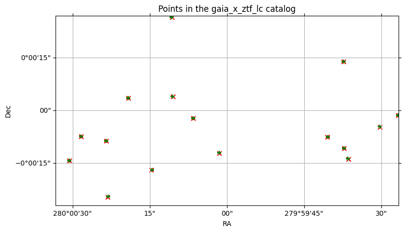
Earlier, we plotted the points for both of the input catalogs. We can plot the points of the output catalog, now, to see how well the crossmatch aligned. Since each row contains the combination of columns from both input catalogs, each row includes the (ra, dec) points from each source catalog, for each row representing a match.

In our case, this means (ra_gaia, dec_gaia) and (objra_ztf_lc, objdec_ztf_lc).

NOTE: we are using the catalog objects, not the computed results, for the plotting, because .plot_points() is a method on the catalog, not on the NestedFrame.

See the plotting tutorial for this technique as well as others.

%%time

# First the Gaia points
gaia_x_ztf.plot_points(
    ra_column="ra_gaia",
    dec_column="dec_gaia",
    center=center,
    fov=fov,
    c="red",
    marker="x",
    s=40,
    label="gaia points",
)

gaia_x_ztf.plot_points(
    ra_column="objra_ztf_lc",
    dec_column="objdec_ztf_lc",
    # Can skip the center & fov args here, since this is an overlay
    c="green",
    marker="+",
    s=30,
    label="ztf points",
)

CPU times: user 4.23 s, sys: 2.19 s, total: 6.42 s
Wall time: 1min 32s

(<Figure size 900x500 with 1 Axes>,
 <WCSAxes: title={'center': 'Points in the gaia_x_ztf_lc catalog'}>)

2.1.2 ztf X gaia (denser on the left)

Now let’s crossmatch the same catalogs, but switching the left and right catalog. Now we have the denser catalog on the left.

The algorithm is, in pseudocode:

for every point in the left catalog:
    find the closest match in the right catalog

When there are more points in the left catalog than in the right, as in this case, each object in the right catalog will get matched to more than one object in the left.

ztf_x_gaia = ztf22_sm.crossmatch(gaia3_sm)
ztf_x_gaia

lsdb Catalog ztf_lc_x_gaia:

	objectid_ztf_lc	objra_ztf_lc	objdec_ztf_lc	nepochs_ztf_lc	lc_ztf_lc	source_id_gaia	ra_gaia	dec_gaia	parallax_gaia	phot_g_n_obs_gaia	phot_g_mean_mag_gaia	_dist_arcsec
npartitions=1
Order: 6, Pixel: 30357	int64[pyarrow]	float[pyarrow]	float[pyarrow]	int64[pyarrow]	nested<hmjd: [double], mag: [float], magerr: [...	int64[pyarrow]	double[pyarrow]	double[pyarrow]	double[pyarrow]	int16[pyarrow]	float[pyarrow]	double[pyarrow]

12 out of 12 columns in the catalog have been loaded lazily, meaning no data has been read, only the catalog schema

%%time
c_ztf_x_gaia = ztf_x_gaia.compute()
c_ztf_x_gaia

CPU times: user 2.25 s, sys: 1.13 s, total: 3.39 s
Wall time: 48 s

	objectid_ztf_lc	objra_ztf_lc	objdec_ztf_lc	nepochs_ztf_lc	lc_ztf_lc	source_id_gaia	ra_gaia	dec_gaia	parallax_gaia	phot_g_n_obs_gaia	phot_g_mean_mag_gaia	_dist_arcsec
2136230505053800416	435313300083261	280.000458	-0.003345	155	hmjd mag magerr 58955.48525 19.895302 0.114786 +154 rows ... ...	4272460980177200768	280.000432	-0.003361	0.306259	102	20.670609	0.126400
2136230505053837760	435213300004409	280.000427	-0.003351	100	hmjd mag magerr 58280.34025 21.346365 0.202767 +99 rows ... ...	4272460980177200768	280.000432	-0.003361	0.306259	102	20.670609	0.038935
2136230505914872355	435313300048086	279.993469	-0.003805	144	hmjd mag magerr 58956.44194 19.609255 0.094674 +143 rows ... ...	4272460980182044416	279.993450	-0.003846		61	20.738001	0.162300
2136230505917728684	435213300027202	279.993408	-0.003810	62	hmjd mag magerr 58275.38118 21.402374 0.206694 +61 rows ... ...	4272460980182044416	279.993450	-0.003846		61	20.738001	0.179975
2136230507991369988	1481208400000483	280.006409	-0.006818	18	hmjd mag magerr 59424.35363 20.744385 0.156009 +17 rows ... ...	4272461018841217920	280.006446	-0.006851	-0.070988	164	20.329275	0.155598
...	...	...	...	...	...	...

47 rows x 12 columns

47 matches in this case, vs 16 matches in the first case. Let’s look at the plot again:

%%time

# First the ZTF points
ztf_x_gaia.plot_points(
    ra_column="objra_ztf_lc",
    dec_column="objdec_ztf_lc",
    center=center,
    fov=fov,
    c="red",
    marker="x",
    s=30,
    label="ztf points",
)

# Then the Gaia points
ztf_x_gaia.plot_points(
    ra_column="ra_gaia",
    dec_column="dec_gaia",
    # Can skip the center & fov args here, since this is an overlay
    c="green",
    marker="+",
    s=40,
    label="gaia points",
)

CPU times: user 4.06 s, sys: 2.09 s, total: 6.15 s
Wall time: 1min 33s

(<Figure size 900x500 with 1 Axes>,
 <WCSAxes: title={'center': 'Points in the ztf_lc_x_gaia catalog'}>)

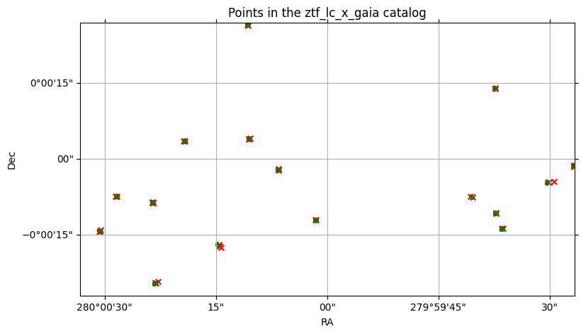
There are several red x markers (left) for each green + marker (right).

And yet, out of the 129 points in the ZTF cone, only 47 of those could be considered matches at all; the other 82 aren’t even candidates.

2.2 Effect of n_neighbors on number of results

One of the arguments to .crossmatch is n_neighbors, which defaults to 1, meaning that for each object in the left catalog, we’re looking for one best match from the right catalog.

But we can look for more than one best match. By increasing this argument, we can get gaia X ztf to produce the same results as ztf X gaia.

gaia_x_ztf_n10 = gaia3_sm.crossmatch(ztf22_sm, n_neighbors=10)
c_gaia_x_ztf_n10 = gaia_x_ztf_n10.compute()
len(c_gaia_x_ztf_n10)

47

47 results, just like ztf x gaia with n_neighbors=1.

2.3 Verifying object identifiers

Converting the catalog identifiers from the crossmatches to Python sets makes it easy to verify that we’ve got not only the right count but the same results. We’re showing that the computed gaia X ztf crossmatch with 10 neighbors produces the same set of results as the computed ztf X gaia crossmatch with 1 neighbor.

gaia_x_ztf_n10_pairs = set(map(tuple, c_gaia_x_ztf_n10[["source_id_gaia", "objectid_ztf_lc"]].to_numpy()))
print("Number of unique matching pairs in gaia X ztf, using 10 neighbors:", len(gaia_x_ztf_n10_pairs))
ztf_x_gaia_n1_pairs = set(map(tuple, c_ztf_x_gaia[["source_id_gaia", "objectid_ztf_lc"]].to_numpy()))
print("Number of unique matching pairs in ztf X gaia, using 1 neighbor:", len(ztf_x_gaia_n1_pairs))

Number of unique matching pairs in gaia X ztf, using 10 neighbors: 47
Number of unique matching pairs in ztf X gaia, using 1 neighbor: 47

# Check that the content of both sets is the same
gaia_x_ztf_n10_pairs == ztf_x_gaia_n1_pairs

True

Closing the Dask client

client.close()

About

Authors: Derek Jones

Last updated on: Oct 27, 2025

If you use lsdb for published research, please cite following instructions.