Cross-match ZTF BTS and NGC

In this notebook, we demonstrate how to cross-match Zwicky Transient Facility (ZTF) Bright Transient Survey (BTS) and New General Catalogue (NGC) using LSDB.

We are using the original survey datasets, as presented by the original survey providers, instead of catalogs that have already been converted to HATS format.

# Install astroquery, comment this line if you already have it
%pip install --quiet astroquery

Note: you may need to restart the kernel to use updated packages.

import lsdb
import matplotlib.pyplot as plt
import numpy as np
import pandas as pd
from astropy.coordinates import SkyCoord
from astropy.table import Table
from astroquery.vizier import Vizier
from dask.distributed import Client

1. Download data

1.1. Download ZTF BTS and convert coordinates to degrees

We download the ZTF BTS data via HTTP, but must first convert the coordinates into degrees before loading as LSDB catalogs.

Of course ZTF looks much deeper than NGC galaxies from 19th century, so we filter ZTF transients by redshift.

%%time

ztf_bts = pd.read_csv(
    "http://sites.astro.caltech.edu/ztf/bts/explorer.php?format=csv",
    na_values="-",
)
ztf_bts = ztf_bts.query("redshift < 0.01")
coord = SkyCoord(ztf_bts["RA"], ztf_bts["Dec"], unit=("hourangle", "deg"))
ztf_bts["ra_deg"], ztf_bts["dec_deg"] = coord.ra.deg, coord.dec.deg
ztf_bts

CPU times: user 61.6 ms, sys: 18.5 ms, total: 80.1 ms
Wall time: 3.42 s

	ZTFID	IAUID	RA	Dec	peakt	peakfilt	peakmag	peakabs	duration	rise	fade	type	redshift	b	A_V	ra_deg	dec_deg
228	ZTF18acbwaxk	SN2018hna	12:26:12.08	+58:18:50.8	503.03	r	13.9583	-16.13	61.205	48.696	12.509	SN II	0.00240	58.502394	0.031	186.550333	58.314111
232	ZTF18acbvgqw	SN2018htt	03:06:02.90	-15:36:41.7	441.75	g	13.9113	-19.07	25.333	10.316	15.017	SN Ia	0.00867	-56.742964	0.101	46.512083	-15.611583
...	...	...	...	...	...	...	...	...	...	...	...	...	...	...	...	...	...
9447	ZTF25aaugeio	SN2025mvn	13:13:27.85	+36:35:11.6	2850.78	r	15.3985	-15.11	>25.08	>15.06	>10.02	SN II	0.00291	79.453892	0.032	198.366042	36.586556
9477	ZTF25aauvber	SN2025ngs	15:35:16.68	+30:51:55.7	2847.77	r	15.5015	-16.73	>19.561	6.481	>13.08	SN II	0.00630	54.177709	0.078	233.819500	30.865472

108 rows × 17 columns

1.2. Download NGC with astroquery

Please install astroquery first with pip install astroquery or conda install -c conda-forge astroquery.

%%time

vizier = Vizier(row_limit=50_000)
tables = vizier.get_catalogs("VII/118/ngc2000")
ngc = tables[0].to_pandas()
coord = SkyCoord(ngc["RAB2000"], ngc["DEB2000"], unit=("hourangle", "deg"))
ngc["ra_deg"], ngc["dec_deg"] = coord.ra.deg, coord.dec.deg
ngc

CPU times: user 685 ms, sys: 15.9 ms, total: 701 ms
Wall time: 702 ms

	Name	Type	RAB2000	DEB2000	Source	Const	l_size	size	mag	n_mag	Desc	ra_deg	dec_deg
0	I5370	Gx	00 00.1	+32 45	m	And		0.7	15.0	p	pB, S, R, stell N	0.025	32.750000
1	I5371		00 00.2	+32 49	d	And		NaN	NaN		F, vS, *15 att	0.050	32.816667
...	...	...	...	...	...	...	...	...	...	...	...	...	...
13224	7807	Gx	23 59.6	-18 51	c	Cet		1.0	NaN		eF, pS, iF	359.900	-18.850000
13225	I5369		23 59.8	+32 41	d	And		NaN	NaN		F, S, R, N	359.950	32.683333

13226 rows × 13 columns

2. Plan cross-match job

LSDB is built upon Dask and can be used with Dask distributed cluster. In this cell we just plan computations and do not actually run them.

%%time

matched_catalog = lsdb.crossmatch(
    ztf_bts,
    ngc,
    radius_arcsec=1200,
    ra_column="ra_deg",
    dec_column="dec_deg",
    suffixes=("_ztf", "_ngc"),
)
matched_catalog

CPU times: user 3.64 s, sys: 287 ms, total: 3.92 s
Wall time: 3.85 s

lsdb Catalog _ztf_x__ngc:

	ZTFID_ztf	IAUID_ztf	RA_ztf	Dec_ztf	peakt_ztf	peakfilt_ztf	peakmag_ztf	peakabs_ztf	duration_ztf	rise_ztf	fade_ztf	type_ztf	redshift_ztf	b_ztf	A_V_ztf	ra_deg_ztf	dec_deg_ztf	Name_ngc	Type_ngc	RAB2000_ngc	DEB2000_ngc	Source_ngc	Const_ngc	l_size_ngc	size_ngc	mag_ngc	n_mag_ngc	Desc_ngc	ra_deg_ngc	dec_deg_ngc	_dist_arcsec
npartitions=10
Order: 0, Pixel: 0	string[pyarrow]	string[pyarrow]	string[pyarrow]	string[pyarrow]	double[pyarrow]	string[pyarrow]	double[pyarrow]	double[pyarrow]	string[pyarrow]	string[pyarrow]	string[pyarrow]	string[pyarrow]	double[pyarrow]	double[pyarrow]	double[pyarrow]	double[pyarrow]	double[pyarrow]	string[pyarrow]	string[pyarrow]	string[pyarrow]	string[pyarrow]	string[pyarrow]	string[pyarrow]	string[pyarrow]	float[pyarrow]	float[pyarrow]	string[pyarrow]	string[pyarrow]	double[pyarrow]	double[pyarrow]	double[pyarrow]
Order: 0, Pixel: 1	...	...	...	...	...	...	...	...	...	...	...	...	...	...	...	...	...	...	...	...	...	...	...	...	...	...	...	...	...	...	...
...	...	...	...	...	...	...	...	...	...	...	...	...	...	...	...	...	...	...	...	...	...	...	...	...	...	...	...	...	...	...	...
Order: 7, Pixel: 161010	...	...	...	...	...	...	...	...	...	...	...	...	...	...	...	...	...	...	...	...	...	...	...	...	...	...	...	...	...	...	...
Order: 7, Pixel: 179663	...	...	...	...	...	...	...	...	...	...	...	...	...	...	...	...	...	...	...	...	...	...	...	...	...	...	...	...	...	...	...

31 out of 31 available columns in the catalog have been loaded lazily, meaning no data has been read, only the catalog schema

3. Run LSDB pipeline

We create a dask client to run the crossmatch in parallel.

Additional Help

For additional information on dask client creation, please refer to the official Dask documentation and our Dask cluster configuration page for LSDB-specific tips. Note that dask also provides its own best practices, which may also be useful to consult.

%%time

# Create default local cluster
with Client():
    matched_df = matched_catalog.compute()

# Let's output transient name, NGC name and angular distance between them
matched_df = matched_df[["IAUID_ztf", "Name_ngc", "_dist_arcsec", "RA_ztf", "Dec_ztf"]].sort_values(
    by=["_dist_arcsec"]
)
matched_df

CPU times: user 342 ms, sys: 93.9 ms, total: 436 ms
Wall time: 3.83 s

	IAUID_ztf	Name_ngc	_dist_arcsec	RA_ztf	Dec_ztf
_healpix_29
1957242016251976064	SN2022xxf	3705	2.985601	11:30:05.93	+09:16:57.2
1827616204711960889	SN2024jlf	5690	6.309787	14:37:42.32	+02:17:04.1
...	...	...	...	...	...
190562289935449883	AT2020aabh	206	1081.99822	00:39:30.06	+40:31:00.8
184639843781841134	AT2022qpg	224	1193.179125	00:44:20.78	+41:23:10.8

84 rows × 5 columns

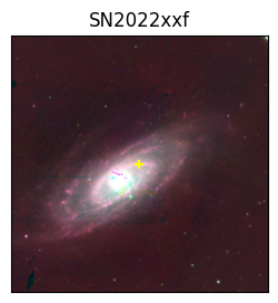
We may have some false matches here, because NGC is too shallow for this task. However, if we sort the table by the cross-match distance, we can see the first one is a supernova (SN2022xxf) in the nearby galaxy NGC 3705.

4. Make some plot

This part is not related to LSDB and adopted from PanSTARRS image this tutorial.

Now let’s download host galaxy image from the PanSTARRS survey and plot it out (with SN location in the middle and marked with a “+”)

def getimages(ra, dec, size=240, filters="grizy"):
    """Query ps1filenames.py service to get a list of images

    ra, dec = position in degrees
    size = image size in pixels (0.25 arcsec/pixel)
    filters = string with filters to include
    Returns a table with the results
    """

    service = "https://ps1images.stsci.edu/cgi-bin/ps1filenames.py"
    url = ("{service}?ra={ra}&dec={dec}&size={size}&format=fits" "&filters={filters}").format(**locals())
    table = Table.read(url, format="ascii")
    return table


def get_ps1_image(url, size=240):
    """
    size: pixel number for 0.25 arcsec/pixel
    """
    from PIL import Image
    import requests
    from io import BytesIO

    try:
        r = requests.get(url)
        im = Image.open(BytesIO(r.content))
    except:
        print("Can't get ps1 image")
        im = None
    return im

c = SkyCoord(
    matched_df["RA_ztf"].to_numpy()[0], matched_df["Dec_ztf"].to_numpy()[0], unit=("hourangle", "deg")
)
ra = c.ra.degree
dec = c.dec.degree
oid = matched_df["IAUID_ztf"].to_numpy()[0]
table = getimages(ra, dec, size=1200, filters="grizy")
url = (
    "https://ps1images.stsci.edu/cgi-bin/fitscut.cgi?"
    "ra={}&dec={}&size=1200&format=jpg&red={}&green={}&blue={}"
).format(ra, dec, table["filename"][0], table["filename"][1], table["filename"][2])
im = get_ps1_image(url)
fig, ax = plt.subplots(figsize=(7, 3))
if im is not None:
    ax.imshow(im)
    ax.set_xticks([])
    ax.set_yticks([])
    ax.scatter(np.average(plt.xlim()), np.average(plt.ylim()), marker="+", color="yellow")
    ax.set_title(oid)
    plt.show()

About

Authors: Konstantin Malanchev, Mi Dai

Last updated on: Oct 27, 2025

If you use lsdb for published research, please cite following instructions.