The Catalog Object

In this tutorial, we will:

• explore the purpose and scope of the Catalog object in an LSDB pipeline

• load catalogs in LSDB and inspect their metadata

Introduction

The Catalog object encapsulates all of the information that LSDB knows about an astronomical catalog, and is the basis for performing operations on the underlying catalog data.

There are two types of catalog data that the Catalog object exposes:

1. high-level metadata: The columns and table schema of the catalog, the number of partitions of data, sky coverage, provenance information, basic aggregate statistics about the data.

2. leaf-level tabular data: the full rows of data from the objects and/or observations in the catalog.

1. Getting Data into LSDB

The simplest way to load a catalog in LSDB is to call lsdb.open_catalog() with a path to a catalog in the HATS format. This will return a Catalog object with all the high level metadata loaded that LSDB needs to enable you to work with the catalog. We recommend you to visit our website, data.lsdb.io, where you are able to find large surveys in HATS format publicly available to use. If you’re looking for how to get your own external data into LSDB, see the topic Import Catalogs instead.

Let’s open GAIA DR3 as an example and take a look at the object we get back.

import lsdb

gaia_path = "https://data.lsdb.io/hats/gaia_dr3"
gaia = lsdb.open_catalog(gaia_path)
gaia

lsdb Catalog gaia:

	solution_id	designation	source_id	random_index	ref_epoch	ra	ra_error	dec	dec_error	parallax	parallax_error	parallax_over_error	pm	pmra	pmra_error	pmdec	pmdec_error	ra_dec_corr	ra_parallax_corr	ra_pmra_corr	ra_pmdec_corr	dec_parallax_corr	dec_pmra_corr	dec_pmdec_corr	parallax_pmra_corr	parallax_pmdec_corr	pmra_pmdec_corr	astrometric_n_obs_al	astrometric_n_obs_ac	astrometric_n_good_obs_al	astrometric_n_bad_obs_al	astrometric_gof_al	astrometric_chi2_al	astrometric_excess_noise	astrometric_excess_noise_sig	astrometric_params_solved	astrometric_primary_flag	nu_eff_used_in_astrometry	pseudocolour	pseudocolour_error	ra_pseudocolour_corr	dec_pseudocolour_corr	parallax_pseudocolour_corr	pmra_pseudocolour_corr	pmdec_pseudocolour_corr	astrometric_matched_transits	visibility_periods_used	astrometric_sigma5d_max	matched_transits	new_matched_transits	matched_transits_removed	ipd_gof_harmonic_amplitude	ipd_gof_harmonic_phase	ipd_frac_multi_peak	ipd_frac_odd_win	ruwe	scan_direction_strength_k1	scan_direction_strength_k2	scan_direction_strength_k3	scan_direction_strength_k4	scan_direction_mean_k1	scan_direction_mean_k2	scan_direction_mean_k3	scan_direction_mean_k4	duplicated_source	phot_g_n_obs	phot_g_mean_flux	phot_g_mean_flux_error	phot_g_mean_flux_over_error	phot_g_mean_mag	phot_bp_n_obs	phot_bp_mean_flux	phot_bp_mean_flux_error	phot_bp_mean_flux_over_error	phot_bp_mean_mag	phot_rp_n_obs	phot_rp_mean_flux	phot_rp_mean_flux_error	phot_rp_mean_flux_over_error	phot_rp_mean_mag	phot_bp_rp_excess_factor	phot_bp_n_contaminated_transits	phot_bp_n_blended_transits	phot_rp_n_contaminated_transits	phot_rp_n_blended_transits	phot_proc_mode	bp_rp	bp_g	g_rp	radial_velocity	radial_velocity_error	rv_method_used	rv_nb_transits	rv_nb_deblended_transits	rv_visibility_periods_used	rv_expected_sig_to_noise	rv_renormalised_gof	rv_chisq_pvalue	rv_time_duration	rv_amplitude_robust	rv_template_teff	rv_template_logg	rv_template_fe_h	rv_atm_param_origin	vbroad	vbroad_error	vbroad_nb_transits	grvs_mag	grvs_mag_error	grvs_mag_nb_transits	rvs_spec_sig_to_noise	phot_variable_flag	l	b	ecl_lon	ecl_lat	in_qso_candidates	in_galaxy_candidates	non_single_star	has_xp_continuous	has_xp_sampled	has_rvs	has_epoch_photometry	has_epoch_rv	has_mcmc_gspphot	has_mcmc_msc	in_andromeda_survey	classprob_dsc_combmod_quasar	classprob_dsc_combmod_galaxy	classprob_dsc_combmod_star	teff_gspphot	teff_gspphot_lower	teff_gspphot_upper	logg_gspphot	logg_gspphot_lower	logg_gspphot_upper	mh_gspphot	mh_gspphot_lower	mh_gspphot_upper	distance_gspphot	distance_gspphot_lower	distance_gspphot_upper	azero_gspphot	azero_gspphot_lower	azero_gspphot_upper	ag_gspphot	ag_gspphot_lower	ag_gspphot_upper	ebpminrp_gspphot	ebpminrp_gspphot_lower	ebpminrp_gspphot_upper	libname_gspphot
npartitions=2016
Order: 2, Pixel: 0	int64[pyarrow]	string[pyarrow]	int64[pyarrow]	int64[pyarrow]	double[pyarrow]	double[pyarrow]	float[pyarrow]	double[pyarrow]	float[pyarrow]	double[pyarrow]	float[pyarrow]	float[pyarrow]	float[pyarrow]	double[pyarrow]	float[pyarrow]	double[pyarrow]	float[pyarrow]	float[pyarrow]	float[pyarrow]	float[pyarrow]	float[pyarrow]	float[pyarrow]	float[pyarrow]	float[pyarrow]	float[pyarrow]	float[pyarrow]	float[pyarrow]	int16[pyarrow]	int16[pyarrow]	int16[pyarrow]	int16[pyarrow]	float[pyarrow]	float[pyarrow]	float[pyarrow]	float[pyarrow]	int8[pyarrow]	bool[pyarrow]	float[pyarrow]	float[pyarrow]	float[pyarrow]	float[pyarrow]	float[pyarrow]	float[pyarrow]	float[pyarrow]	float[pyarrow]	int16[pyarrow]	int16[pyarrow]	float[pyarrow]	int16[pyarrow]	int16[pyarrow]	int16[pyarrow]	float[pyarrow]	float[pyarrow]	int8[pyarrow]	int8[pyarrow]	float[pyarrow]	float[pyarrow]	float[pyarrow]	float[pyarrow]	float[pyarrow]	float[pyarrow]	float[pyarrow]	float[pyarrow]	float[pyarrow]	bool[pyarrow]	int16[pyarrow]	double[pyarrow]	float[pyarrow]	float[pyarrow]	float[pyarrow]	int16[pyarrow]	double[pyarrow]	float[pyarrow]	float[pyarrow]	float[pyarrow]	int16[pyarrow]	double[pyarrow]	float[pyarrow]	float[pyarrow]	float[pyarrow]	float[pyarrow]	int16[pyarrow]	int16[pyarrow]	int16[pyarrow]	int16[pyarrow]	int8[pyarrow]	float[pyarrow]	float[pyarrow]	float[pyarrow]	float[pyarrow]	float[pyarrow]	int8[pyarrow]	int16[pyarrow]	int16[pyarrow]	int16[pyarrow]	float[pyarrow]	float[pyarrow]	float[pyarrow]	float[pyarrow]	float[pyarrow]	float[pyarrow]	float[pyarrow]	float[pyarrow]	int16[pyarrow]	float[pyarrow]	float[pyarrow]	int16[pyarrow]	float[pyarrow]	float[pyarrow]	int16[pyarrow]	float[pyarrow]	string[pyarrow]	double[pyarrow]	double[pyarrow]	double[pyarrow]	double[pyarrow]	bool[pyarrow]	bool[pyarrow]	int16[pyarrow]	bool[pyarrow]	bool[pyarrow]	bool[pyarrow]	bool[pyarrow]	bool[pyarrow]	bool[pyarrow]	bool[pyarrow]	bool[pyarrow]	float[pyarrow]	float[pyarrow]	float[pyarrow]	float[pyarrow]	float[pyarrow]	float[pyarrow]	float[pyarrow]	float[pyarrow]	float[pyarrow]	float[pyarrow]	float[pyarrow]	float[pyarrow]	float[pyarrow]	float[pyarrow]	float[pyarrow]	float[pyarrow]	float[pyarrow]	float[pyarrow]	float[pyarrow]	float[pyarrow]	float[pyarrow]	float[pyarrow]	float[pyarrow]	float[pyarrow]	string[pyarrow]
Order: 2, Pixel: 1	...	...	...	...	...	...	...	...	...	...	...	...	...	...	...	...	...	...	...	...	...	...	...	...	...	...	...	...	...	...	...	...	...	...	...	...	...	...	...	...	...	...	...	...	...	...	...	...	...	...	...	...	...	...	...	...	...	...	...	...	...	...	...	...	...	...	...	...	...	...	...	...	...	...	...	...	...	...	...	...	...	...	...	...	...	...	...	...	...	...	...	...	...	...	...	...	...	...	...	...	...	...	...	...	...	...	...	...	...	...	...	...	...	...	...	...	...	...	...	...	...	...	...	...	...	...	...	...	...	...	...	...	...	...	...	...	...	...	...	...	...	...	...	...	...	...	...	...	...	...	...	...
...	...	...	...	...	...	...	...	...	...	...	...	...	...	...	...	...	...	...	...	...	...	...	...	...	...	...	...	...	...	...	...	...	...	...	...	...	...	...	...	...	...	...	...	...	...	...	...	...	...	...	...	...	...	...	...	...	...	...	...	...	...	...	...	...	...	...	...	...	...	...	...	...	...	...	...	...	...	...	...	...	...	...	...	...	...	...	...	...	...	...	...	...	...	...	...	...	...	...	...	...	...	...	...	...	...	...	...	...	...	...	...	...	...	...	...	...	...	...	...	...	...	...	...	...	...	...	...	...	...	...	...	...	...	...	...	...	...	...	...	...	...	...	...	...	...	...	...	...	...	...	...	...
Order: 3, Pixel: 766	...	...	...	...	...	...	...	...	...	...	...	...	...	...	...	...	...	...	...	...	...	...	...	...	...	...	...	...	...	...	...	...	...	...	...	...	...	...	...	...	...	...	...	...	...	...	...	...	...	...	...	...	...	...	...	...	...	...	...	...	...	...	...	...	...	...	...	...	...	...	...	...	...	...	...	...	...	...	...	...	...	...	...	...	...	...	...	...	...	...	...	...	...	...	...	...	...	...	...	...	...	...	...	...	...	...	...	...	...	...	...	...	...	...	...	...	...	...	...	...	...	...	...	...	...	...	...	...	...	...	...	...	...	...	...	...	...	...	...	...	...	...	...	...	...	...	...	...	...	...	...	...
Order: 3, Pixel: 767	...	...	...	...	...	...	...	...	...	...	...	...	...	...	...	...	...	...	...	...	...	...	...	...	...	...	...	...	...	...	...	...	...	...	...	...	...	...	...	...	...	...	...	...	...	...	...	...	...	...	...	...	...	...	...	...	...	...	...	...	...	...	...	...	...	...	...	...	...	...	...	...	...	...	...	...	...	...	...	...	...	...	...	...	...	...	...	...	...	...	...	...	...	...	...	...	...	...	...	...	...	...	...	...	...	...	...	...	...	...	...	...	...	...	...	...	...	...	...	...	...	...	...	...	...	...	...	...	...	...	...	...	...	...	...	...	...	...	...	...	...	...	...	...	...	...	...	...	...	...	...	...

152 out of 152 available columns in the catalog have been loaded lazily, meaning no data has been read, only the catalog schema

Additional Help

For tips on accessing remote data, see our Accessing remote data guide

The Gaia catalog is very wide so you would be requesting its whole set of >150 columns. We can see all of the columns available in the catalog by using the all_columns property.

gaia.all_columns[:10]  # Truncating the output to not display the whole list

['solution_id',
 'designation',
 'source_id',
 'random_index',
 'ref_epoch',
 'ra',
 'ra_error',
 'dec',
 'dec_error',
 'parallax']

Note that it’s important (and highly recommended) to:

• Pre-select a small subset of columns that satisfies your scientific needs. Loading an unnecessarily large amount of data leads to computationally expensive and inefficient workflows. To see which columns are available, use the catalog.all_columns property, then load the catalog with only the necesarry columns.

• Load catalogs with their respective margin caches, when available. These margins are necessary to obtain accurate results in several operations such as joining and crossmatching. If you’re working with catalogs from data.lsdb.io, the margin cache will be included in the open_catalog() call for you to copy if it is available. For more information about margins please visit our Margins topic notebook.

Let’s define the set of columns we need and add the margin catalog’s path to our open_catalog call.

gaia = lsdb.open_catalog(
    "https://data.lsdb.io/hats/gaia_dr3/",
    columns=[
        "source_id",
        "ra",
        "dec",
        "phot_g_mean_mag",
        "phot_proc_mode",
        "azero_gspphot",
        "classprob_dsc_combmod_star",
    ],
)
gaia

lsdb Catalog gaia:

	source_id	ra	dec	phot_g_mean_mag	phot_proc_mode	azero_gspphot	classprob_dsc_combmod_star
npartitions=2016
Order: 2, Pixel: 0	int64[pyarrow]	double[pyarrow]	double[pyarrow]	float[pyarrow]	int8[pyarrow]	float[pyarrow]	float[pyarrow]
Order: 2, Pixel: 1	...	...	...	...	...	...	...
...	...	...	...	...	...	...	...
Order: 3, Pixel: 766	...	...	...	...	...	...	...
Order: 3, Pixel: 767	...	...	...	...	...	...	...

7 out of 152 available columns in the catalog have been loaded lazily, meaning no data has been read, only the catalog schema

When we look at the catalog’s representation above, we can see all the columns that are in the catalog object along with their datatypes, and information about how HATS has partitioned the catalog. But there’s one thing that we can’t see: we haven’t loaded any of the data yet! That’s why we have the ... as placeholders for the data, and the warning at the bottom. This is because LSDB’s operations are what we call lazy: they don’t actually perform any work on the data when you call them, they just plan out the pipeline of operations to be performed later. This is how LSDB can work on huge catalogs with billions of rows, and run on any scale of device from a laptop up to a supercomputer. To learn more about how Lazy operations work, take a look at our lazy operations tutorial.

2. Inspecting the Catalog metadata

The natural next step once you have a catalog object is to explore the metadata that has been loaded to understand what kind of data is inside your catalog.

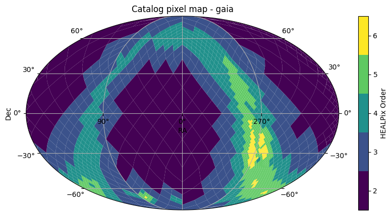
First, we will generate a basic plot showing the sky coverage of the catalog. The Catalog object’s plot_pixels method shows a plot of the HATS partitioning of the catalog. GAIA is a survey that covers the whole sky, so we see the whole sky covered in pixels. The colors of the pixels represent the pixel sizes. The main advantage of HATS partitioning is that the partitions all contain roughly the same amount of rows, so the smaller the pixels, the more dense the catalog is in that area. This explains why we see smaller pixels in the galactic bulge.

gaia.plot_pixels()

(<Figure size 1000x500 with 2 Axes>,
 <WCSAxes: title={'center': 'Catalog pixel map - gaia'}>)

We can also get an idea of the schema of data that’s stored in the catalog, by looking at the columns and dtypes.

gaia.columns

Index(['source_id', 'ra', 'dec', 'phot_g_mean_mag', 'phot_proc_mode',
       'azero_gspphot', 'classprob_dsc_combmod_star'],
      dtype='object')

gaia.dtypes

source_id                      int64[pyarrow]
ra                            double[pyarrow]
dec                           double[pyarrow]
phot_g_mean_mag                float[pyarrow]
phot_proc_mode                  int8[pyarrow]
azero_gspphot                  float[pyarrow]
classprob_dsc_combmod_star     float[pyarrow]
dtype: object

The columns method shows the columns that have been loaded, and will be available to any operations on the catalog. You can still see all of the columns in the catalog by calling the all_columns method, but to use any of these columns that aren’t in the columns the catalog will need to be opened again with these columns selected.

gaia.all_columns[:10]  # Truncating the output to not display the whole list

['solution_id',
 'designation',
 'source_id',
 'random_index',
 'ref_epoch',
 'ra',
 'ra_error',
 'dec',
 'dec_error',
 'parallax']

We can also see how many objects are in the catalog, which is another piece of metadata that is loaded by open_catalog.

len(gaia)

1812731847

Working with Catalog Data

Now that we have a catalog object, we’re ready to start planning and executing operations on the data! Our next tutorials will explain how that works and all the operations you can do with LSDB.

About

Authors: Sandro Campos, Melissa DeLucchi, and Sean McGuire

Last updated/verified on: Jan 19, 2026

If you use lsdb for published research, please cite following instructions.