Working with Time Series Data

Working with Time Series Data#

Learning objectives#

In this tutorial, we will:

count and filter data containing time-series points
apply functions to time-series data and filter both individual points and entire rows based on the results

You should already have an understanding of:

nested-pandas (see https://nested-pandas.readthedocs.io/en/latest/)

Introduction#

Each object in a row has columns that describe the properties of that object. In the case of catalogs with time series data, some columns are lists, having many points per object, each with their own properties, and one of those properties is time. Thus each object has data describing measurements over time.

Moreover, each row may have a different number of data points in its time series, meaning that it can be a ragged data set. One common use case of this capability, which we will explore in this tutorial, is to store and process an object’s light curve.

This structure creates some challenges, because at times you need to filter and operate on the rows as a whole, and sometimes you need to filter and operate on the points that make up the light curves. These operations can further change the number of points within each light curve. lsdb and nested_pandas make this workflow possible in a compact and efficient way.

Open a catalog#

Additional Help

For additional information on dask client creation, please refer to the official Dask documentation and our Dask cluster configuration page for LSDB-specific tips. Note that dask also provides its own best practices, which may also be useful to consult.

For tips on accessing remote data, see our Accessing remote data guide

[1]:

import lsdb

[2]:

from dask.distributed import Client

# Will be used implicitly for all distributed operations
client = Client(n_workers=4, memory_limit="auto")

The ZTF DR 22 catalog contains light curve data, with multiple time points for each object. It’s good practice to work with a small part of the catalog first, by using a cone search, say, before running computations across all of its partitions.

Note that the lightcurve data appears as list types in the schema.

[3]:

ztf_objects = lsdb.open_catalog(
    "https://data.lsdb.io/hats/ztf_dr22",
    search_filter=lsdb.ConeSearch(ra=254.5, dec=35.3, radius_arcsec=1800),
)
ztf_objects

[3]:

lsdb Catalog ztf_lc:

	objectid	filterid	objra	objdec	nepochs	hmjd	mag	magerr	clrcoeff	catflags
npartitions=1
Order: 5, Pixel: 2378	int64[pyarrow]	int8[pyarrow]	float[pyarrow]	float[pyarrow]	int64[pyarrow]	list<element: double>[pyarrow]	list<element: float>[pyarrow]	list<element: float>[pyarrow]	list<element: float>[pyarrow]	list<element: int32>[pyarrow]

10 out of 15 available columns in the catalog have been loaded lazily, meaning no data has been read, only the catalog schema

1. The time series light curve data#

These list types, the columns which describe the light curve data, are (from https://irsa.ipac.caltech.edu/data/ZTF/docs/releases/dr22/ztf_release_notes_dr22.pdf):

hmjd (Heliocentric-based Modified Julian Date)
mag (Calibrated magnitude for a source)
magerr (Corresponding 1-σ uncertainty in mag estimate)
clrcoeff (Linear color coefficient term from photometric calibration)
catflags (Photometric/image quality flags encoded as bits)

Regarding catflags, Note 9b in the above document states: “If you demand perfectly clean extractions at every epoch, we advise specifying catflags = 0 when querying lightcurve epochs.” We will do that in this tutorial.

What this means is that the nepochs column, which specifies how many points there are in the list columns, will not be a reliable count following filtering. We will address this following filtering.

1.1 Nesting the light curve data#

Rather than continue to deal with the list columns as individual lists, it is much more tractable to create a nested column out of them, so that all of the lightcurve data is grouped together, visually and computationally. The .nest_lists method does this.

Afterward, we’ll peek at the top three rows using .head().

[4]:

%%time
ztf_objects = ztf_objects.nest_lists(
    list_columns=["hmjd", "mag", "magerr", "clrcoeff", "catflags"],
    name="lc",  # name to give the resulting nested column
)
ztf_objects.head(3)

CPU times: user 4.62 s, sys: 1.65 s, total: 6.26 s
Wall time: 1min 30s

[4]:

objectid

filterid

objra

objdec

nepochs

lc

669362595299170956

1722203100001567

2

254.563019

34.803379

1

hmjd	mag	magerr	clrcoeff	catflags
58294.3155	21.090492	0.183403	0.09443	0
+0 rows	...	...	...	...

669362595506888097

681212200003914

2

254.564301

34.804192

32

hmjd	mag	magerr	clrcoeff	catflags
58198.49622	21.547998	0.238883	0.104513	0
+31 rows	...	...	...	...

669362595508866719

1722203100001554

2

254.564240

34.804264

6

hmjd	mag	magerr	clrcoeff	catflags
58292.29516	21.082235	0.18281	0.095064	0
+5 rows	...	...	...	...

3 rows x 6 columns

Note that in the preview above, the number of light curve points for each object is different.

Note further that throughout most of this notebook, the operations we request are delayed. They aren’t computed until .compute() is called, or until a preview function, like .head().

1.2 Querying (filtering) the time series data in the nested column#

Now the nested column lc contains all of the time series data. We want to only keep the perfectly clear observations, those with lc.catflags == 0. The .query() method, when used on nested columns, goes inside the nest, keeping only those nested rows which satisfy the condition.

We’d also like to focus on the r-band only, which is filterid == 2. This column is not nested, but applies to every point in the lightcurve. This also means that we can’t query it in the same expression as the catflags, that is, we cannot write .query("filterid == 2 and lc.catflags == 0"), because that kind of cross-nest filtering isn’t supported yet.

But we can accomplish the identical effect by simply chaining the two queries.

[5]:

filtered_catalog = ztf_objects.query("filterid == 2")
filtered_catalog = filtered_catalog.query("lc.catflags == 0")

This filtering may have completely removed all of the points from some objects’ light curves. Drop rows for which this is true.

[ ]:

# Using map_partitions to drop rows with NaN in lc.mag
filtered_catalog = filtered_catalog.map_partitions(lambda df: df.dropna(subset=["lc.mag"]))

2. Analysis of time series data#

Let’s compute the period of each time series with a Lomb-Scargle periodogram. As a prerequisite, we want to use as input only brighter points, those where the median magnitude is brighter than 16.

We want to compute a new column named median_mag which contains the median magnitude, which is not nested (it will apply to the entire row), and we want to add this column to our catalog. We will use the .map_rows function, which is so named because it allows us to map a function onto each row of the catalog, pulling in all column values and nested information.

Some things to note about the code here:

We use append_columns=True, because we want the new columns to be appended to our existing columns (rather than creating a new single-column catalog).
For every input column provided, the user-defined function must have a parameter which will receive that column. We only provide one here, called "lc.mag", and so median_mag only takes a single argument.
We are obliged to provide meta=, which is a description of the type of our new column(s), and includes each column’s name and type. This is a requirement when using .map_rows().

[ ]:

import numpy as np


def median_mag(row):
    return np.median(row["lc.mag"])
    # return {"median_mag": np.median(row["lc.mag"])}


catalog_w_features = filtered_catalog.map_rows(
    median_mag,  # our user-defined function
    columns=["lc.mag"],  # names of the column(s) to pass to the function
    output_names=["median_mag"],  # name(s) of the new column(s)
    meta={"median_mag": float},  # for Dask: describe the type of the output
    append_columns=True,
)
catalog_w_features

lsdb Catalog ztf_lc:

	objectid	filterid	objra	objdec	nepochs	lc	median_mag
npartitions=1
Order: 5, Pixel: 2378	int64[pyarrow]	int8[pyarrow]	float[pyarrow]	float[pyarrow]	int64[pyarrow]	nested<hmjd: [double], mag: [float], magerr: [...	float64

7 out of 15 available columns in the catalog have been loaded lazily, meaning no data has been read, only the catalog schema

Note that the resulting catalog_w_features has our new columns, median_mag, at the right. We can now use this to filter rows (including the time series nested with each row under lc) using .query():

[8]:

catalog_w_features = catalog_w_features.query("median_mag < 16")

We’d also like to ignore time series data that has fewer than 10 detections.

We can’t use nepochs for anymore, since it included observations for which catflags != 0. What we’ll do instead is use a function from nested_pandas called count_nested, which is able to count all of the points per nested field. This function adds a column to its input, named n_{column}, or n_lc in this case, since we’re counting the length of the sub-columns within lc.

We’ll apply this function using .map_partitions, which, like .map_rows, applies a function in parallel across the partitions of the catalog, but with a slightly different syntax.

Note that we don’t need to supply meta= to .map_partitions. This is because count_nested correctly handles the case of an empty input, producing an empty output with the right structure.

Now that the catalog has the new column n_lc, we can filter out any time series data having fewer than 10 detections.

[9]:

from nested_pandas.utils import count_nested


def count_points(pts):
    # Asked to count `lc`, this will add a column called `n_lc`
    return count_nested(pts, "lc")


catalog_w_features = catalog_w_features.map_partitions(count_points)
catalog_w_features = catalog_w_features.query("n_lc >= 10")

2.1 Applying the periodogram to the qualifying time series data#

Now we’ve got good data for computing a periodogram! The data now has these properties:

perfectly clean extractions (lc.catflags == 0)
r-band only (filterid == 2)
median of lc.mag is brighter than 16
at least 10 points

Once again, we’ll use Catalog.map_rows to map a function onto each row (each timeseries) and produce two new columns for our catalog:

period (the period of the peridogram)
false_alarm_prob (the probability that the periodogram peak arose from noise rather than a true signal, and is hence a false alarm)

Since Lomb-Scargle requires time, magnitude, and magnitude error, we need to pass these three inputs to it.

[10]:

from astropy.timeseries import LombScargle


def extract_period(row):
    time = row["lc.hmjd"]
    mag = row["lc.mag"]
    error = row["lc.magerr"]
    ls = LombScargle(time, mag, error)
    freq, power = ls.autopower()
    argmax = np.argmax(power)
    period = 1.0 / freq[argmax]
    false_alarm_prob = ls.false_alarm_probability(power[argmax])
    return {"period": period, "false_alarm_prob": false_alarm_prob}


catalog_w_features = catalog_w_features.map_rows(
    extract_period,
    # Column names specifying function arguments
    columns=["lc.hmjd", "lc.mag", "lc.magerr"],
    # Returned data type shape
    meta={"period": float, "false_alarm_prob": float},
    append_columns=True,
)
catalog_w_features

[10]:

lsdb Catalog ztf_lc:

	objectid	filterid	objra	objdec	nepochs	lc	median_mag	n_lc	period	false_alarm_prob
npartitions=1
Order: 5, Pixel: 2378	int64[pyarrow]	int8[pyarrow]	float[pyarrow]	float[pyarrow]	int64[pyarrow]	nested<hmjd: [double], mag: [float], magerr: [...	float64	int32	float64	float64

10 out of 15 available columns in the catalog have been loaded lazily, meaning no data has been read, only the catalog schema

Now we have everything we need to be able to select light curves by their period. Let’s focus on those without a false alarm which are close to having a period between 1.5 and 9.5.

Note that because both of these columns are at the same nesting level (the base) we can run the query with logical operators like and.

[11]:

periodic_catalog = catalog_w_features.query("false_alarm_prob < 1e-10 and 1.5 < period < 9.5")

2.2 Computing and plotting#

Operations have run suspiciously quickly so far because no computation has been done yet, only some validation of structure while Dask builds the task graph invisibly. We can now realize the computation by calling .compute().

[12]:

%%time
periodic_df = periodic_catalog.compute()
periodic_df

/Users/dbranton/.virtualenvs/lsdb/lib/python3.12/site-packages/numpy/_core/fromnumeric.py:3596: RuntimeWarning: Mean of empty slice.
  return _methods._mean(a, axis=axis, dtype=dtype,
/Users/dbranton/.virtualenvs/lsdb/lib/python3.12/site-packages/numpy/_core/_methods.py:138: RuntimeWarning: invalid value encountered in divide
  ret = ret.dtype.type(ret / rcount)

CPU times: user 4.98 s, sys: 1.67 s, total: 6.64 s
Wall time: 1min 42s

[12]:

objectid

filterid

objra

objdec

nepochs

lc

median_mag

n_lc

period

false_alarm_prob

669389465489798434

680209200002339

2

254.245834

34.911369

1495

hmjd	mag	magerr	clrcoeff	catflags
58198.39514	15.919156	0.012013	0.094193	0
+1396 rows	...	...	...	...

15.911603

1397

5.714512

0.000000

669411015865751384

680213300009232

2

254.457520

35.342350

1403

hmjd	mag	magerr	clrcoeff	catflags
58198.39511	14.103342	0.015016	0.08511	0
+1312 rows	...	...	...	...

13.564873

1313

1.700147

0.000000

669558955615458377

681216300004749

2

254.589752

35.765709

1545

hmjd	mag	magerr	clrcoeff	catflags
58198.42248	15.413739	0.010634	0.079598	0
+1451 rows	...	...	...	...

15.388121

1452

8.966459

0.000000

3 rows x 10 columns

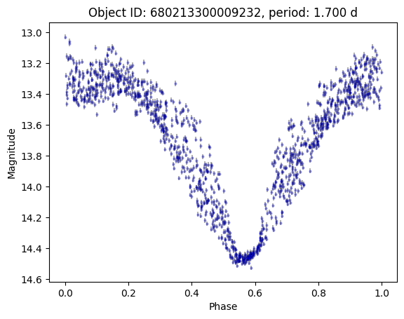
Only a few! The one with 1313 points is HZ Her, a bright X-ray binary system. Let’s plot it.

[13]:

import matplotlib.pyplot as plt

row = periodic_df.iloc[1]
lc = row.lc

peak_mjd = lc["hmjd"][lc["mag"].idxmin()]
lc["phase"] = (lc["hmjd"] - peak_mjd) % row.period / row.period

plt.errorbar(
    lc["phase"],
    lc["mag"],
    lc["magerr"],
    alpha=0.3,
    ls="none",
    marker="o",
    markersize=2,
    markeredgecolor="blue",
    color="black",
)
plt.gca().invert_yaxis()
plt.xlabel("Phase")
plt.ylabel("Magnitude")
plt.title(f"Object ID: {row.objectid}, period: {row.period:.3f} d")

[13]:

Text(0.5, 1.0, 'Object ID: 680213300009232, period: 1.700 d')

../../_images/tutorials_pre_executed_timeseries_32_1.png

Close the Dask client#

[14]:

client.close()

About#

Author(s): Konstantin Malanchev, Derek Jones

Last updated on: Oct 27, 2025

If you use lsdb for published research, please cite following instructions.

Working with Time Series Data

Contents

Working with Time Series Data#

Learning objectives#

Introduction#

Open a catalog#

1. The time series light curve data#

1.1 Nesting the light curve data#

1.2 Querying (filtering) the time series data in the nested column#

2. Analysis of time series data#

2.1 Applying the periodogram to the qualifying time series data#

2.2 Computing and plotting#

Close the Dask client#

About#