Get light-curves from ZTF and PS1 for SNAD catalog#
This notebook demonstrates how to get epoch photometry for a custom pointing catalog, in this case, the SNAD catalog. We will get the SNAD catalog as a pandas dataframe, cross-match it with PS1 DR2 object (OTMO) “detection” catalogs and ZTF DR16 Zubercal catalog.
1. Install and import required packages#
[1]:
# Install lsdb and matplotlib
%pip install --quiet lsdb matplotlib
Note: you may need to restart the kernel to use updated packages.
[2]:
import dask.distributed
import matplotlib.pyplot as plt
import numpy as np
import pandas as pd

from lsdb import open_catalog, from_dataframe
from upath import UPath
2. Load catalogs#
2.1. Define paths to PS1 DR2 catalogs#
We access all the data through the web, so we don’t need to download it in advance. However, we are going much more data than we’re actually going to use, so it will take some time.
Additional Help
For tips on accessing remote data, see our Accessing remote data tutorial
[3]:
# Define paths to PS1 DR2 catalogs
PS1_PATH = UPath("s3://stpubdata/panstarrs/ps1/public/hats/", anon=True)
PS1_OBJECT = PS1_PATH / "otmo"
PS1_DETECTION = PS1_PATH / "detection"

# Define paths to ZTF DR16 Zubercal catalog
ZUBERCAL_PATH = "https://data.lsdb.io/hats/ztf_dr16/zubercal/"
2.2. Download and convert SNAD catalog to LSDB format, in memory#
SNAD catalog is just ~100 rows, we download it through Pandas and convert to LSDB’s Catalog object with lsdb.from_dataframe.
[4]:
# Load SNAD catalog, remove rows with missing values and rename columns to more friendly names
snad_df = pd.read_csv(
    "https://snad.space/catalog/snad_catalog.csv",
    dtype_backend="pyarrow",
).dropna()
display(snad_df)

# Convert to LSDB's Catalog object
snad_catalog = from_dataframe(
    snad_df,
    # Optimize partition size
    drop_empty_siblings=True,
    # Keep partitions small
    lowest_order=5,
    # Specify columns with coordinates
    ra_column="R.A.",
    dec_column="Dec.",
)
display(snad_catalog)
| Name | R.A. | Dec. | OID | Discovery date (UT) | mag | er_down | er_up | ref | er_ref | TNS/VSX | Type | Comments | |
|---|---|---|---|---|---|---|---|---|---|---|---|---|---|
| 0 | SNAD101 | 247.45543 | 24.77282 | 633207400004730 | 2018-04-08 09:45:49 | 21.11 | 0.27 | 0.36 | 20.84 | 0.06 | AT 2018lwh | PSN | ZTF18abqkqdm |
| 1 | SNAD102 | 245.05375 | 28.3822 | 633216300024691 | 2018-03-21 11:08:19 | 21.18 | 0.28 | 0.39 | 20.26 | 0.07 | AT 2018lwi | PSN | ZTF18abdgwos |
| ... | ... | ... | ... | ... | ... | ... | ... | ... | ... | ... | ... | ... | ... |
| 185 | SNAD287 | 243.77243 | 8.83445 | 533202300011210 | 2018-05-08 09:15:11 | 20.1 | 0.16 | 0.19 | 19.61 | 0.05 | AT 2018mps | PSN | ZTF19aaltuxk |
| 186 | SNAD288 | 17.1193 | 31.16565 | 650202200001826 | 2022-03-02 02:52:47 | 20.89 | 0.25 | 0.32 | 20.9 | 0.1 | AT 2022aezi | AGN | ZTF22abeuuvu |
120 rows × 13 columns
| Name | R.A. | Dec. | OID | Discovery date (UT) | mag | er_down | er_up | ref | er_ref | TNS/VSX | Type | Comments | |
|---|---|---|---|---|---|---|---|---|---|---|---|---|---|
| npartitions=113 | |||||||||||||
| Order: 7, Pixel: 3996 | string[pyarrow] | double[pyarrow] | double[pyarrow] | int64[pyarrow] | string[pyarrow] | double[pyarrow] | double[pyarrow] | double[pyarrow] | string[pyarrow] | double[pyarrow] | string[pyarrow] | string[pyarrow] | string[pyarrow] |
| Order: 7, Pixel: 8902 | ... | ... | ... | ... | ... | ... | ... | ... | ... | ... | ... | ... | ... |
| ... | ... | ... | ... | ... | ... | ... | ... | ... | ... | ... | ... | ... | ... |
| Order: 5, Pixel: 8184 | ... | ... | ... | ... | ... | ... | ... | ... | ... | ... | ... | ... | ... |
| Order: 7, Pixel: 144952 | ... | ... | ... | ... | ... | ... | ... | ... | ... | ... | ... | ... | ... |
2.3. Load PS1 catalog structure and metadata#
lsdb.open_catalog doesn’t load the data immediately, it just reads the metadata and structure of the catalog. Here we use it to load PS1 DR2 object and detection catalogs, selecting only a few columns to speed up the pipeline.
[5]:
# Load PS1 catalogs metadata
ps1_object = open_catalog(
    PS1_OBJECT,
    columns=[
        "objID",  # PS1 ID
        "raMean",
        "decMean",  # coordinates to use for cross-matching
        "nStackDetections",  # some other data to use
    ],
)
display(ps1_object)

ps1_detection = open_catalog(
    PS1_DETECTION,
    columns=[
        "objID",  # PS1 object ID
        "detectID",  # PS1 detection ID
        # not really going to use it, but we can alternatively directly cross-match with detection table
        "ra",
        "dec",
        # light-curve stuff
        "obsTime",
        "filterID",
        "psfFlux",
        "psfFluxErr",
    ],
)
display(ps1_detection)
| objID | raMean | decMean | nStackDetections | |
|---|---|---|---|---|
| npartitions=27161 | ||||
| Order: 5, Pixel: 0 | int64[pyarrow] | double[pyarrow] | double[pyarrow] | int16[pyarrow] |
| Order: 5, Pixel: 1 | ... | ... | ... | ... |
| ... | ... | ... | ... | ... |
| Order: 6, Pixel: 49150 | ... | ... | ... | ... |
| Order: 6, Pixel: 49151 | ... | ... | ... | ... |
| objID | detectID | ra | dec | obsTime | filterID | psfFlux | psfFluxErr | |
|---|---|---|---|---|---|---|---|---|
| npartitions=83004 | ||||||||
| Order: 6, Pixel: 0 | int64[pyarrow] | int64[pyarrow] | double[pyarrow] | double[pyarrow] | double[pyarrow] | int16[pyarrow] | double[pyarrow] | double[pyarrow] |
| Order: 6, Pixel: 1 | ... | ... | ... | ... | ... | ... | ... | ... |
| ... | ... | ... | ... | ... | ... | ... | ... | ... |
| Order: 6, Pixel: 49150 | ... | ... | ... | ... | ... | ... | ... | ... |
| Order: 6, Pixel: 49151 | ... | ... | ... | ... | ... | ... | ... | ... |
2.4. Load ZTF DR16 Zubercal catalog#
Zubercal is a uber-calibrated light-curve catalog for ZTF DR16. It matches ZTF detections to PS1 objects and provides calibrated magnitudes.
[6]:
# Load Zubercal metadata
zubercal = open_catalog(
    ZUBERCAL_PATH,
    columns=[
        "objectid",  # matches to PS1 objID
        "mjd",
        "band",
        "mag",
        "magerr",  # integer, units are 1e-4 mag
    ],
)
display(zubercal)
| objectid | mjd | band | mag | magerr | objra | objdec | |
|---|---|---|---|---|---|---|---|
| npartitions=70853 | |||||||
| Order: 5, Pixel: 0 | int64[pyarrow] | double[pyarrow] | string[pyarrow] | float[pyarrow] | uint16[pyarrow] | float[pyarrow] | float[pyarrow] |
| Order: 5, Pixel: 1 | ... | ... | ... | ... | ... | ... | ... |
| ... | ... | ... | ... | ... | ... | ... | ... |
| Order: 6, Pixel: 49150 | ... | ... | ... | ... | ... | ... | ... |
| Order: 6, Pixel: 49151 | ... | ... | ... | ... | ... | ... | ... |
3. Plan cross-matching and joining#
LSDB doesn’t do any work until you call compute method, so here we just plan the work.
We find PS1 objects that are within 1 arcsec of SNAD objects.
Join Zubercal catalog to aggregate light-curves. Each light-curve would be represented by a “nested” dataframe, where each row is a detection.
Do the same for PS1 detections.
[7]:
# Planning cross-matching with objects, no work happens here
snad_ps1 = snad_catalog.crossmatch(
    ps1_object,
    radius_arcsec=0.2,
    suffixes=["", ""],
    suffix_method="overlapping_columns",
    # Ignore the missing margin cache.
    # Theoretically it may cause some data loss, but not in this pipeline
    require_right_margin=False,
)

# Join with Zubercal detections to get one more set of light-curves
snad_ztf_lc = snad_ps1.join_nested(
    zubercal,
    left_on="objID",
    right_on="objectid",
    # light-curve will live in "ztf_lc" column
    nested_column_name="ztf_lc",
    output_catalog_name="snad_ztf_lc",
)

# Join with PS1 detections to get light-curves
snad_ps1_ztf_lc = snad_ztf_lc.join_nested(
    ps1_detection,
    left_on="objID",
    right_on="objID",
    # light-curve will live in "ps1_lc" column
    nested_column_name="ps1_lc",
    output_catalog_name="snad_ps1_ztf_lc",
)

display(snad_ps1_ztf_lc)
/astro/users/olynn/lsdb/src/lsdb/dask/crossmatch_catalog_data.py:160: RuntimeWarning: Right catalog does not have a margin cache. Results may be incomplete and/or inaccurate.
  warnings.warn(
/astro/users/olynn/lsdb/src/lsdb/dask/join_catalog_data.py:390: RuntimeWarning: Right catalog does not have a margin cache. Results may be incomplete and/or inaccurate.
  warnings.warn(
/astro/users/olynn/lsdb/src/lsdb/dask/join_catalog_data.py:390: RuntimeWarning: Right catalog does not have a margin cache. Results may be incomplete and/or inaccurate.
  warnings.warn(
| Name | R.A. | Dec. | OID | Discovery date (UT) | mag | er_down | er_up | ref | er_ref | TNS/VSX | Type | Comments | objID | raMean | decMean | nStackDetections | _dist_arcsec | ztf_lc | ps1_lc | |
|---|---|---|---|---|---|---|---|---|---|---|---|---|---|---|---|---|---|---|---|---|
| npartitions=120 | ||||||||||||||||||||
| Order: 7, Pixel: 3996 | string[pyarrow] | double[pyarrow] | double[pyarrow] | int64[pyarrow] | string[pyarrow] | double[pyarrow] | double[pyarrow] | double[pyarrow] | string[pyarrow] | double[pyarrow] | string[pyarrow] | string[pyarrow] | string[pyarrow] | int64[pyarrow] | double[pyarrow] | double[pyarrow] | int16[pyarrow] | double[pyarrow] | nested<mjd: [double], band: [string], mag: [fl... | nested<detectID: [int64], ra: [double], dec: [... |
| Order: 7, Pixel: 8902 | ... | ... | ... | ... | ... | ... | ... | ... | ... | ... | ... | ... | ... | ... | ... | ... | ... | ... | ... | ... |
| ... | ... | ... | ... | ... | ... | ... | ... | ... | ... | ... | ... | ... | ... | ... | ... | ... | ... | ... | ... | ... |
| Order: 7, Pixel: 130954 | ... | ... | ... | ... | ... | ... | ... | ... | ... | ... | ... | ... | ... | ... | ... | ... | ... | ... | ... | ... |
| Order: 7, Pixel: 144952 | ... | ... | ... | ... | ... | ... | ... | ... | ... | ... | ... | ... | ... | ... | ... | ... | ... | ... | ... | ... |
4. Run the pipeline!#
Here we finally run the pipeline and get the light-curves. This requires Dask client for parallel execution, and you probably want to adjust the parameters to your hardware.
The output ndf is a nested dataframe, NestedFrame from nested-pandas package. We will see later how to access the light-curves from it.
Additional Help
For additional information on dask client creation, please refer to the official Dask documentation and our Dask cluster configuration page for LSDB-specific tips. Note that dask also provides its own best practices, which may also be useful to consult.
[8]:
%%time

# It will take a way to fetch all the data from the Internet
with dask.distributed.Client() as client:
    display(client)
    ndf = snad_ps1_ztf_lc.compute()

display(ndf)
/astro/users/olynn/.conda/envs/p311/lib/python3.11/site-packages/distributed/node.py:187: UserWarning: Port 8787 is already in use.
Perhaps you already have a cluster running?
Hosting the HTTP server on port 34979 instead
  warnings.warn(
Client
Client-88bdaa19-b34b-11f0-8a37-043201587601
| Connection method: Cluster object | Cluster type: distributed.LocalCluster |
| Dashboard: http://127.0.0.1:34979/status |
Cluster Info
LocalCluster
a6eca3fe
| Dashboard: http://127.0.0.1:34979/status | Workers: 16 |
| Total threads: 256 | Total memory: 1.48 TiB |
| Status: running | Using processes: True |
Scheduler Info
Scheduler
Scheduler-ff9a5728-cbb7-4cc2-99ab-1caee04f7894
| Comm: tcp://127.0.0.1:42015 | Workers: 16 |
| Dashboard: http://127.0.0.1:34979/status | Total threads: 256 |
| Started: Just now | Total memory: 1.48 TiB |
Workers
Worker: 0
| Comm: tcp://127.0.0.1:36877 | Total threads: 16 |
| Dashboard: http://127.0.0.1:33279/status | Memory: 94.43 GiB |
| Nanny: tcp://127.0.0.1:34113 | |
| Local directory: /tmp/dask-scratch-space-1515041/worker-emwuewuo | |
Worker: 1
| Comm: tcp://127.0.0.1:33333 | Total threads: 16 |
| Dashboard: http://127.0.0.1:36193/status | Memory: 94.43 GiB |
| Nanny: tcp://127.0.0.1:37101 | |
| Local directory: /tmp/dask-scratch-space-1515041/worker-9nmjm3iv | |
Worker: 2
| Comm: tcp://127.0.0.1:42949 | Total threads: 16 |
| Dashboard: http://127.0.0.1:33425/status | Memory: 94.43 GiB |
| Nanny: tcp://127.0.0.1:33885 | |
| Local directory: /tmp/dask-scratch-space-1515041/worker-xyfdwu99 | |
Worker: 3
| Comm: tcp://127.0.0.1:33795 | Total threads: 16 |
| Dashboard: http://127.0.0.1:36895/status | Memory: 94.43 GiB |
| Nanny: tcp://127.0.0.1:37657 | |
| Local directory: /tmp/dask-scratch-space-1515041/worker-_mmi22u7 | |
Worker: 4
| Comm: tcp://127.0.0.1:34907 | Total threads: 16 |
| Dashboard: http://127.0.0.1:44451/status | Memory: 94.43 GiB |
| Nanny: tcp://127.0.0.1:39213 | |
| Local directory: /tmp/dask-scratch-space-1515041/worker-vs9kc6q4 | |
Worker: 5
| Comm: tcp://127.0.0.1:40255 | Total threads: 16 |
| Dashboard: http://127.0.0.1:39129/status | Memory: 94.43 GiB |
| Nanny: tcp://127.0.0.1:38723 | |
| Local directory: /tmp/dask-scratch-space-1515041/worker-ciqsk583 | |
Worker: 6
| Comm: tcp://127.0.0.1:35549 | Total threads: 16 |
| Dashboard: http://127.0.0.1:44221/status | Memory: 94.43 GiB |
| Nanny: tcp://127.0.0.1:34247 | |
| Local directory: /tmp/dask-scratch-space-1515041/worker-ftvx6b3s | |
Worker: 7
| Comm: tcp://127.0.0.1:45135 | Total threads: 16 |
| Dashboard: http://127.0.0.1:45357/status | Memory: 94.43 GiB |
| Nanny: tcp://127.0.0.1:37459 | |
| Local directory: /tmp/dask-scratch-space-1515041/worker-7blh5dwm | |
Worker: 8
| Comm: tcp://127.0.0.1:42363 | Total threads: 16 |
| Dashboard: http://127.0.0.1:36271/status | Memory: 94.43 GiB |
| Nanny: tcp://127.0.0.1:41529 | |
| Local directory: /tmp/dask-scratch-space-1515041/worker-lcq8n8r5 | |
Worker: 9
| Comm: tcp://127.0.0.1:37341 | Total threads: 16 |
| Dashboard: http://127.0.0.1:46827/status | Memory: 94.43 GiB |
| Nanny: tcp://127.0.0.1:40489 | |
| Local directory: /tmp/dask-scratch-space-1515041/worker-_mdmikuv | |
Worker: 10
| Comm: tcp://127.0.0.1:44567 | Total threads: 16 |
| Dashboard: http://127.0.0.1:36993/status | Memory: 94.43 GiB |
| Nanny: tcp://127.0.0.1:34977 | |
| Local directory: /tmp/dask-scratch-space-1515041/worker-7fqoteed | |
Worker: 11
| Comm: tcp://127.0.0.1:45495 | Total threads: 16 |
| Dashboard: http://127.0.0.1:36931/status | Memory: 94.43 GiB |
| Nanny: tcp://127.0.0.1:38089 | |
| Local directory: /tmp/dask-scratch-space-1515041/worker-ksuj3_x9 | |
Worker: 12
| Comm: tcp://127.0.0.1:41763 | Total threads: 16 |
| Dashboard: http://127.0.0.1:46223/status | Memory: 94.43 GiB |
| Nanny: tcp://127.0.0.1:45927 | |
| Local directory: /tmp/dask-scratch-space-1515041/worker-vvc1ok9m | |
Worker: 13
| Comm: tcp://127.0.0.1:38915 | Total threads: 16 |
| Dashboard: http://127.0.0.1:37803/status | Memory: 94.43 GiB |
| Nanny: tcp://127.0.0.1:43067 | |
| Local directory: /tmp/dask-scratch-space-1515041/worker-4qq7xfll | |
Worker: 14
| Comm: tcp://127.0.0.1:36101 | Total threads: 16 |
| Dashboard: http://127.0.0.1:37643/status | Memory: 94.43 GiB |
| Nanny: tcp://127.0.0.1:33265 | |
| Local directory: /tmp/dask-scratch-space-1515041/worker-ohutsea6 | |
Worker: 15
| Comm: tcp://127.0.0.1:37513 | Total threads: 16 |
| Dashboard: http://127.0.0.1:32837/status | Memory: 94.43 GiB |
| Nanny: tcp://127.0.0.1:33025 | |
| Local directory: /tmp/dask-scratch-space-1515041/worker-hk79nu4y | |
| Name | R.A. | Dec. | OID | Discovery date (UT) | mag | er_down | er_up | ref | er_ref | TNS/VSX | Type | Comments | objID | raMean | decMean | nStackDetections | _dist_arcsec | ztf_lc | ps1_lc | |||||||||||||||||||||||||||||||
|---|---|---|---|---|---|---|---|---|---|---|---|---|---|---|---|---|---|---|---|---|---|---|---|---|---|---|---|---|---|---|---|---|---|---|---|---|---|---|---|---|---|---|---|---|---|---|---|---|---|---|
| 392922938507087610 | SNAD195 | 173.238910 | 47.548460 | 754108100010282 | 2019-05-14 05:00:23 | 20.620000 | 0.200000 | 0.250000 | 20.84 | 0.040000 | AT 2019aapu | PSN | ZTF19aavkyng | 165051732389348889 | 173.238928 | 47.548471 | 5 | 0.058477 |
|
|
||||||||||||||||||||||||||||||
| 425505064326790713 | SNAD283 | 161.377530 | 56.059230 | 787210100006486 | 2023-03-10 05:53:26 | 19.730000 | 0.130000 | 0.150000 | 20.9 | 0.140000 | AT 2023aeeh | PSN | ZTF23aaaptpf | 175271613774741837 | 161.377536 | 56.059198 | 4 | 0.116292 |
|
|
||||||||||||||||||||||||||||||
| 446151138901733801 | SNAD243 | 113.919200 | 31.779590 | 662105400007673 | 2018-03-30 05:34:18 | 20.810000 | 0.280000 | 0.390000 | 19.8 | 0.070000 | AT 2018mdt | PSN | ZTF18aceqval | 146131139191046084 | 113.919172 | 31.779571 | 10 | 0.110847 |
|
|
||||||||||||||||||||||||||||||
| 636762943118841180 | SNAD199 | 232.002550 | 29.723200 | 631115200000919 | 2019-05-29 08:21:26 | 20.090000 | 0.150000 | 0.170000 | 19.99 | 0.070000 | AT 2019aapy | PSN | ZTF19aavovik | 143662320025368377 | 232.002534 | 29.723172 | 5 | 0.112213 |
|
|
||||||||||||||||||||||||||||||
| 636879053204760495 | SNAD225 | 231.084920 | 29.975240 | 677101400006297 | 2018-04-02 08:45:19 | 19.700000 | 0.120000 | 0.140000 | 19.6 | 0.040000 | AT 2018mdb | PSN | ZTF18aajzqbq | 143972310848550829 | 231.084883 | 29.975228 | 5 | 0.121680 |
|
|
||||||||||||||||||||||||||||||
| ... | ... | ... | ... | ... | ... | ... |
CPU times: user 8.93 s, sys: 2.08 s, total: 11 s
Wall time: 5min 2s
5. Plot first five light curves#
Here we plot light curves, you can change plot type by setting MAG_OR_FLUX to mag or flux.
NestedFrame from nested-pandas (docs) is just a wrapper around pandas DataFrame, so all you know about pandas applies here. Every light-curve is packed into items of ps1_lc and ztf_lc columns. When you are getting a single element from a nested dataframe, you get a pandas dataframe!
[9]:
MAG_OR_FLUX = "mag"

ps1_filter_id_to_name = {1: "g", 2: "r", 3: "i", 4: "z", 5: "y"}
get_ps1_name_from_filter_id = np.vectorize(ps1_filter_id_to_name.get)
filter_colors = {"g": "green", "r": "red", "i": "black", "z": "purple", "y": "cyan"}

ndf_sorted = ndf.sort_values("Name")

for i in range(5):
    # snad_name is a string, ps1_lc and ztf_lc are pandas dataframes
    snad_name, ps1_lc, ztf_lc = ndf_sorted.iloc[i][["Name", "ps1_lc", "ztf_lc"]]

    # when we iterate a nested series we are getting pandas dataframes of light curves
    plt.figure(figsize=(12, 6))

    # PS1
    ps1_bands = get_ps1_name_from_filter_id(ps1_lc["filterID"])
    for band in "grizy":
        color = filter_colors[band]
        band_idx = ps1_bands == band
        t = ps1_lc["obsTime"][band_idx]
        flux = ps1_lc["psfFlux"][band_idx] * 1e6  # micro Jy
        err = ps1_lc["psfFluxErr"][band_idx] * 1e6
        mag = 8.9 - 2.5 * np.log10(flux / 1e6)
        mag_plus = 8.9 - 2.5 * np.log10((flux - err) / 1e6)
        mag_minus = 8.9 - 2.5 * np.log10((flux + err) / 1e6)
        if MAG_OR_FLUX == "flux":
            plt.scatter(
                t,
                flux,
                marker="*",
                color=color,
                label=f"PS1 {band}",
                alpha=0.3,
            )
            plt.errorbar(
                t,
                flux,
                err,
                ls="",
                color=color,
                alpha=0.15,
            )
        elif MAG_OR_FLUX == "mag":
            plt.scatter(
                t,
                mag,
                marker="*",
                color=color,
                label=f"PS1 {band}",
                alpha=0.3,
            )
            plt.errorbar(
                t,
                mag,
                [mag - mag_minus, mag_plus - mag],
                ls="",
                color=color,
                alpha=0.15,
            )
        else:
            raise ValueError(f"MAG_OR_FLUX should be mag or flux")

    # ZTF
    ztf_bands = ztf_lc["band"]
    for band in "gri":
        band_idx = ztf_bands == band
        color = filter_colors[band]
        t = ztf_lc["mjd"][band_idx]
        mag = ztf_lc["mag"][band_idx]
        magerr = np.asarray(ztf_lc["magerr"][band_idx], dtype=float) * 1e-4
        flux = np.power(10, 0.4 * (8.9 - mag)) * 1e6  # micro Jy
        err = 0.4 * np.log(10) * flux * magerr
        if MAG_OR_FLUX == "flux":
            plt.scatter(
                t,
                flux,
                marker="x",
                color=color,
                label=f"ZTF {band}",
                alpha=0.3,
            )
            plt.errorbar(
                t,
                flux,
                err,
                ls="",
                color=color,
                alpha=0.15,
            )
        else:
            plt.scatter(
                t,
                mag,
                marker="x",
                color=color,
                label=f"ZTF {band}",
                alpha=0.3,
            )
            plt.errorbar(
                t,
                mag,
                magerr,
                ls="",
                color=color,
                alpha=0.15,
            )

    plt.title(snad_name)
    plt.xlabel("MJD")
    plt.ylabel("Flux, μJy" if MAG_OR_FLUX == "flux" else "mag")
    if MAG_OR_FLUX == "mag":
        plt.gca().invert_yaxis()
    plt.legend(loc="upper left")
/astro/users/olynn/.conda/envs/p311/lib/python3.11/site-packages/matplotlib/cbook.py:1719: FutureWarning: Calling float on a single element Series is deprecated and will raise a TypeError in the future. Use float(ser.iloc[0]) instead
  return math.isfinite(val)
/astro/users/olynn/.conda/envs/p311/lib/python3.11/site-packages/matplotlib/cbook.py:1719: FutureWarning: Calling float on a single element Series is deprecated and will raise a TypeError in the future. Use float(ser.iloc[0]) instead
  return math.isfinite(val)
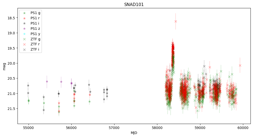
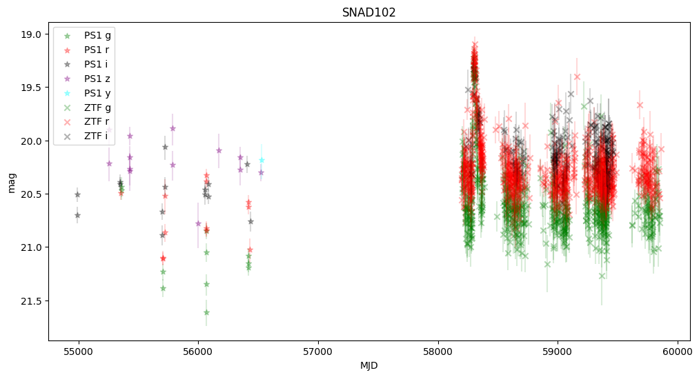
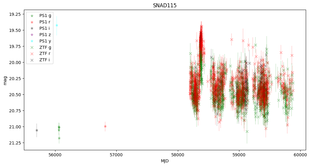
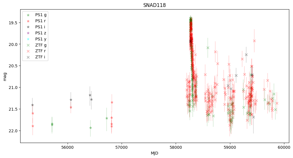
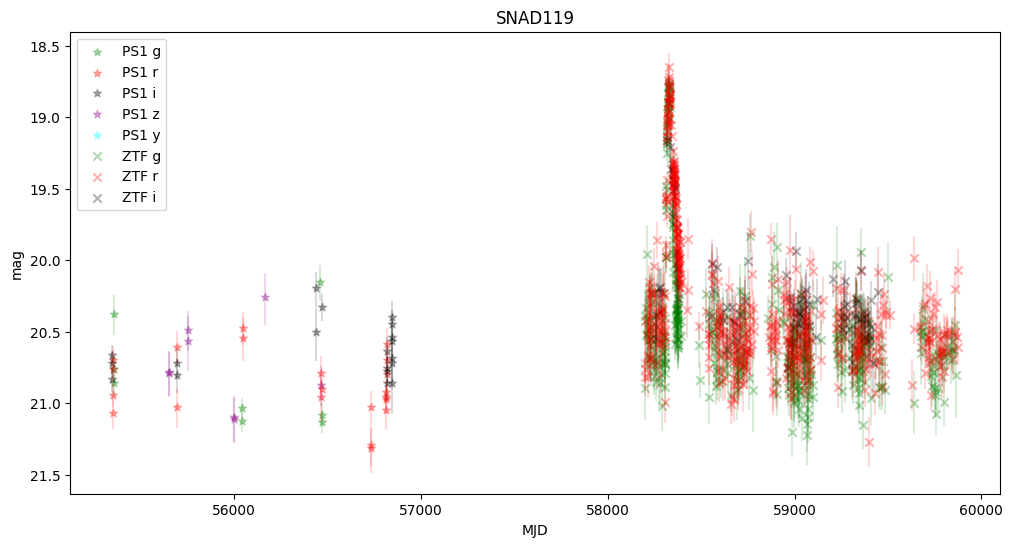
We observe that some objects are missing—this is because Pan-STARRS lacked information about the transients, and the host center is either too faint or too distant from the transient.
None of these objects were active in Pan-STARRS, but they were active in ZTF, confirming that they are robust supernova candidates.
About#
Authors: Konstantin Malanchev
Last updated on: Oct 27, 2025
If you use lsdb for published research, please cite following instructions.